Analysis and Control of a Rotary Inverted Pendulum System (ROTPEN)

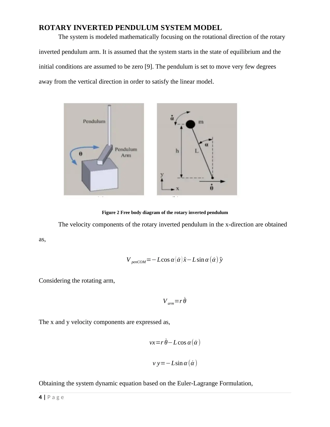
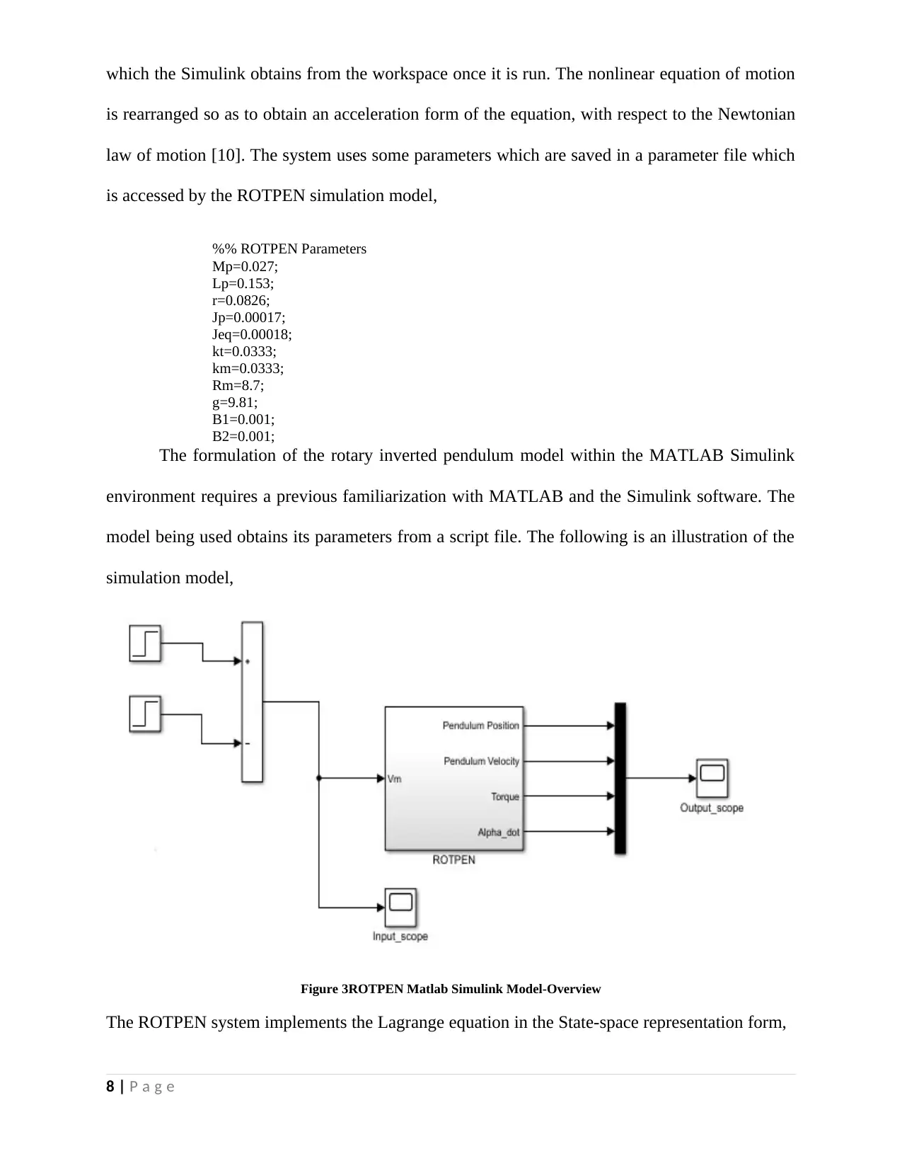
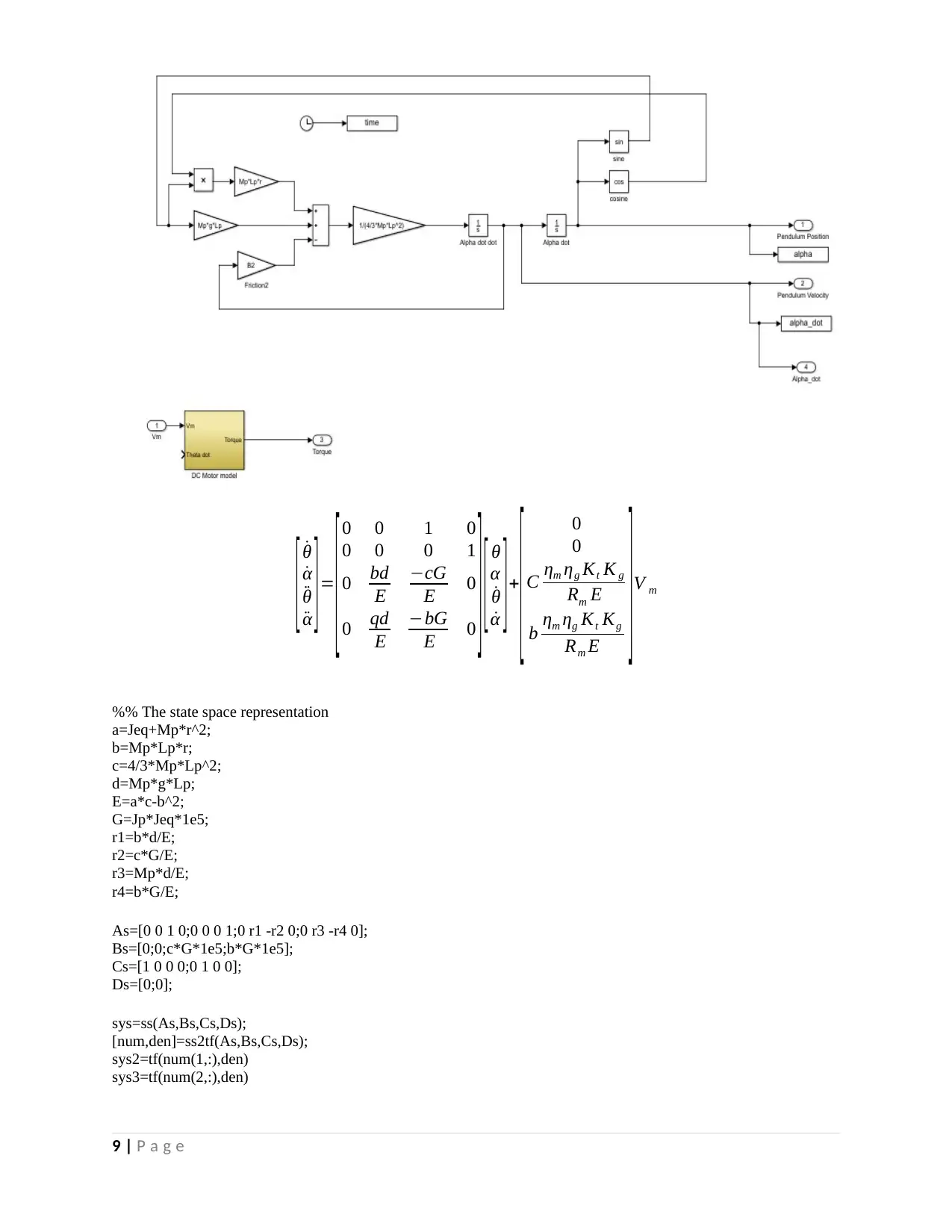
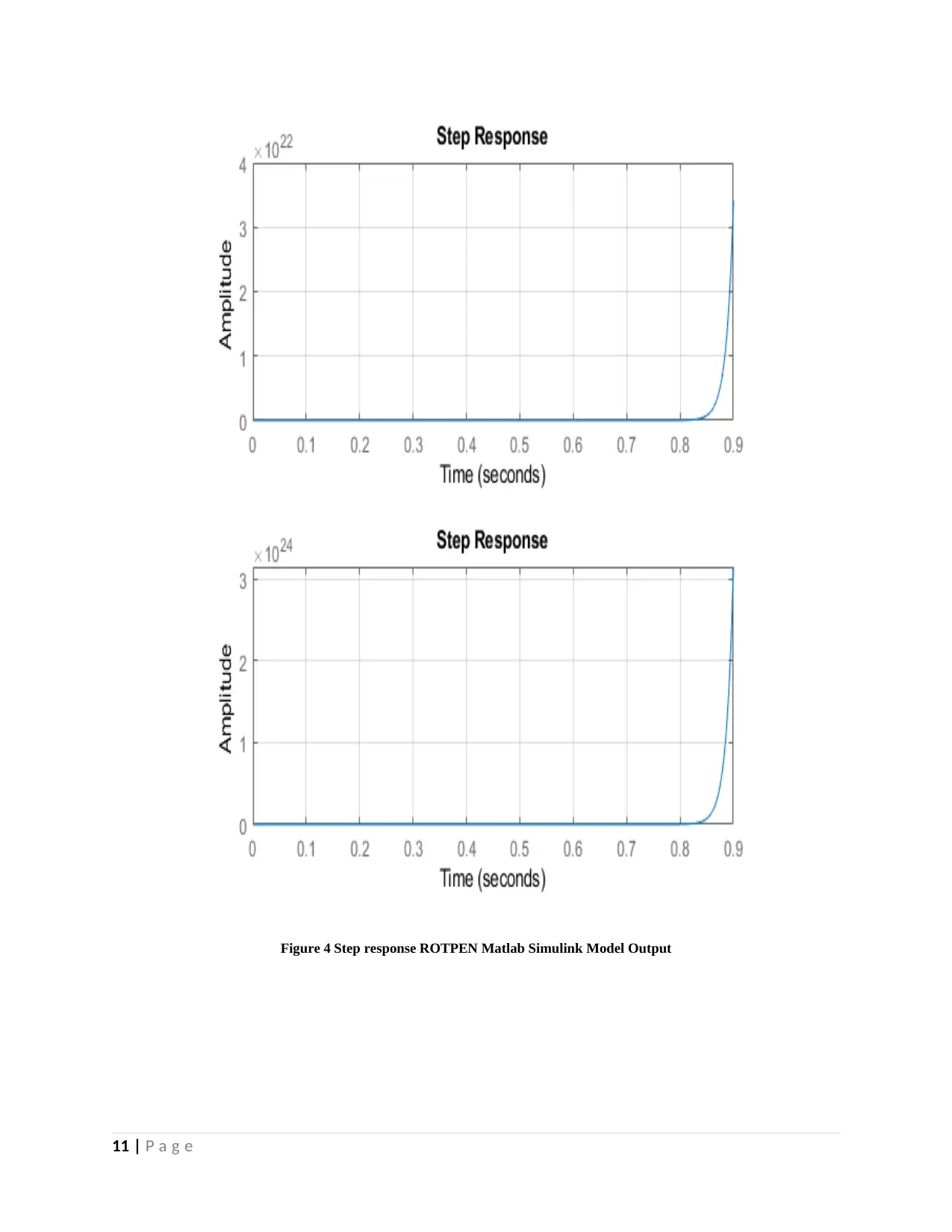
This lab report analyzes the control and instrumentation of a rotary inverted pendulum (ROTPEN) system. The report begins with an introduction to the system and its applications, followed by the aims of the experiment, which include linearizing the nonlinear system, defining its state-space representation, designing a state-feedback controller, and simulating both open-loop and closed-loop systems. The report then details the mathematical modeling of the ROTPEN system, using Euler-Lagrange equations to derive the equations of motion. A Simulink model is developed and discussed, including the parameters, and the state-space representation. Controller design, including open-loop and closed-loop system simulations, and the application of pole placement techniques are presented. The report includes figures illustrating the system's behavior, such as step responses, Bode diagrams, and root locus plots. The discussion section compares different control schemes and the conclusion summarizes the findings and suggests future work. The report also includes references to related literature.

Control & Instrumentation
Lab Assignment
Student Name
Student ID Number
Instructor (professor)
Institutional affiliation
Location(state, country)
Date of submission

TABLE OF CONTENTS
INTRODUCTION...........................................................................................................................1
AIMS OF THE EXPERIMENT......................................................................................................3
ROTARY INVERTED PENDULUM SYSTEM MODEL.............................................................3
ROTARY INVERTED PENDULUM SIMULINK MODEL.........................................................7
CONTROLLER DESIGN...............................................................................................................8
DISCUSSION..................................................................................................................................8
CONCLUSION & FUTURE WORKS...........................................................................................8
REFERENCES................................................................................................................................9
LIST OF FIGURES
Figure 1 ROTPEN rotary inverted pendulum on LABVIEW [source: Quanser].........................................3
Figure 2 Free body diagram of the rotary inverted pendulum......................................................................4
Figure 3ROTPEN Matlab Simulink Model-Overview................................................................................9
Figure 4 Step response ROTPEN Matlab Simulink Model Output............................................................12
Figure 5 Bode Diagram to show magnitude and phase of ROTPEN Pendulum........................................13
Figure 6 Open loop system Simulation Model Block................................................................................14
Figure 7 Root Locus for Transfer Function 1............................................................................................15
Figure 8 Root Locus for transfer function 2...............................................................................................16
Figure 9 Pole location for a closed loop system........................................................................................18
Figure 10 State feedback controller for a closed loop ROTPEN pendulum...............................................18
Figure 11 The ROTPEN controller for the Pendulum link........................................................................19
Figure 12 System Simulation Balance Control Response for the closed loop............................................20
Figure 13 Results form Simulation of the ROTPEN model.......................................................................21
Figure 14 ROTPEN Model........................................................................................................................22
Figure 15 State Feedback controller segment............................................................................................22
1 | P a g e

INTRODUCTION
The rotary inverted pendulum is a nonlinear system whose initial state is unstable hence
the need for control. There are different methods implemented in the control of the rotary
inverted pendulum. In the analysis, the velocity of the pendulum center of mass, is considered for
a system displaced in the angle, a, and in the x-direction [1]-[5]. The system has a motor that
moves the cart along a straight track with the pendulum attached to the cart using a pin joint. The
axis of rotation of the pendulum link is considered to be horizontal and it is perpendicular to the
cart’s direction of motion. The input of the system is the force that is applied to the cart through
the motor. The horizontal link is coupled such that it links directly or by connecting to a gearing
of the motor shaft and the rotary motion [6]. The QNET rotary inverted pendulum kit is
comprised of the dc motor, L-shaped arm, and pendulum, and two optical encoders, Elvis II
board. The motor that runs the pendulum is mounted on a metallic chamber. The pendulum is
suspended on a horizontal axis at the end of the arm. The pendulum and arm angle are measured
by two separate encoders [7]. The control variable is the input voltage to the pulse width
modulated amplifier that controls the motor.
Figure 1 ROTPEN rotary inverted pendulum on LABVIEW [source: Quanser]
2 | P a g e

The rotary inverted pendulum is applied in the industries especially where items need to
be lifted from one point to another. The same system is implemented in robots and in the large
cranes used in the construction industry [8]. In some mall, the system is used to design the
Segway used to by security guards to monitor the premises. The ROTPEN kit in the 2 DOF
freely moves in two rotary directions.
AIMS OF THE EXPERIMENT
(a) To linearize a non-linear rotary inverted pendulum systems using Euler-Lagrange
equations of motion.
(b) To define the linear state-space representation of the rotary inverted pendulum system
(c) To develop a state-feedback or full feedback control to balance the pendulum in the
upright position using a pole placement.
(d) To simulate the open-loop and the closed loop systems of the ROTPEN inverted
pendulum so that the specifications are met and evaluating the performance.
3 | P a g e

ROTARY INVERTED PENDULUM SYSTEM MODEL
The system is modeled mathematically focusing on the rotational direction of the rotary
inverted pendulum arm. It is assumed that the system starts in the state of equilibrium and the
initial conditions are assumed to be zero [9]. The pendulum is set to move very few degrees
away from the vertical direction in order to satisfy the linear model.
Figure 2 Free body diagram of the rotary inverted pendulum
The velocity components of the rotary inverted pendulum in the x-direction are obtained
as,
V penCOM =−Lcos α ( ˙α ) ^x−L sin α ( ˙α ) ^y
Considering the rotating arm,
V arm=r ˙θ
The x and y velocity components are expressed as,
vx=r ˙θ−L cos α ( ˙α )
v y=−Lsin α ( ˙α )
Obtaining the system dynamic equation based on the Euler-Lagrange Formulation,
4 | P a g e

V =P Epend =mgh=mgL cos α
T =K Ehub +K EV x
+ K EV y
+ K Epend
The moment of inertia for a rod is given based on the center of mass, such that,
Jcm=( 1
12 ) M R2
The half of the pendulum length is described as L such that,
R=2 L
Jcm=( 1
12 ) M (2 L)2= ( 1
3 )M L2
The kinetic energy equation can be written as,
T =( 1
2 ) Jeq ˙θ2+ ( 1
2 )m ( r ˙θ−Lcos α ( ˙α ) )2+ ( 1
2 )m (−L sin α ( ˙α ) )2 + (1
2 )Jcm ˙α2
Determining the KE function using the Lagrangian formulation, the equation results into,
L=T −V =( 1
2 )J eq ˙θ2 + ( 2
3 )m L2 ˙α2−mLr cos α ( ˙α ) ( ˙θ ) + (1
2 )m r2 ˙θ2−mgL cos α
The two equations are used to obtain the angular components,
δ
δt ( δL
δ ˙θ )− δL
δθ =T output−Beq ˙θ
δ
δt ( δL
δ ˙α )− δL
δα =0
Linearizing the equation at α=0,
5 | P a g e

( J eq+m r2 ) ¨θ−mLr ¨α=T output−Beq ˙θ
4
3 m L2 ¨α−mLr ¨θ−mgLα=0
The torque of the motor that powers the rotary action of the rotary inverted pendulum is given as,
T output= ηm ηg K t K g ( V m−K G K m ˙θ )
Rm
All the governing equations are combined to represent the complete system operation using the
state space representation below,
[ ˙θ
˙α
¨θ
¨α ]=
[0 0 1 0
0 0 0 1
0 bd
E
−cG
E 0
0 qd
E
−bG
E 0 ] [ θ
α
˙θ
˙α ]+
[ 0
0
C ηm ηg Kt K g
Rm E
b ηm ηg Kt Kg
Rm E ]V m
a=J eq+mr2, b=mLr, c= 4
3 m L2
, d=mgL, E=ac−b2
G= ηm ηg K t K g
2−Beq Rm
Rm
Using the Euler equation of the rotational motion of the pendulum at the pin point, we get the
equation,
JB ¨α=∑ M B → 1
12 m ( 2 L )2 ¨α= Ax Lcos ( α ) + A y L sin ( α )
→ 1
3 m L2 ¨α −Ax Lcos α + A y L sin ( α )
Jo ¨θ=∑ M 0 → J eq ¨θ=T1−Beq ˙θ− Ax r
6 | P a g e

1
3 m L2 ¨α= ( mr ¨θ+mL sin ( α ) ˙α 2−mL cos ( α ) ¨α L cos ( α ) )+ ( mg−mL cos ( α ) ˙α 2−mL sin ( α ) ¨α ) L sin α
→ 1
3 m L2 ¨α= (mLr cos ( α ) ¨θ+m L2 sin ( α ) cos ( α ) ˙α2−m L2 cos2 ( α ) ¨α )+ (mgLsin ( α )−m L2 sin ( α ) cos ( α ) ˙α2−m L2 sin2 ( α
→−mLr cos ( α ) ¨θ+ 4
3 m L2 ¨α−mgLsin ( α )=0
ROTARY INVERTED PENDULUM SIMULINK MODEL
The rotary inverted pendulum Simulink model is developed for a nonlinear system. The
system depends on a MATLAB script that highlights all the values of the system parameters
7 | P a g e

which the Simulink obtains from the workspace once it is run. The nonlinear equation of motion
is rearranged so as to obtain an acceleration form of the equation, with respect to the Newtonian
law of motion [10]. The system uses some parameters which are saved in a parameter file which
is accessed by the ROTPEN simulation model,
%% ROTPEN Parameters
Mp=0.027;
Lp=0.153;
r=0.0826;
Jp=0.00017;
Jeq=0.00018;
kt=0.0333;
km=0.0333;
Rm=8.7;
g=9.81;
B1=0.001;
B2=0.001;
The formulation of the rotary inverted pendulum model within the MATLAB Simulink
environment requires a previous familiarization with MATLAB and the Simulink software. The
model being used obtains its parameters from a script file. The following is an illustration of the
simulation model,
Figure 3ROTPEN Matlab Simulink Model-Overview
The ROTPEN system implements the Lagrange equation in the State-space representation form,
8 | P a g e

[ ˙θ
˙α
¨θ
¨α ]=
[0 0 1 0
0 0 0 1
0 bd
E
−cG
E 0
0 qd
E
−bG
E 0 ] [ θ
α
˙θ
˙α ]+
[ 0
0
C ηm ηg Kt K g
Rm E
b ηm ηg Kt Kg
Rm E ]V m
%% The state space representation
a=Jeq+Mp*r^2;
b=Mp*Lp*r;
c=4/3*Mp*Lp^2;
d=Mp*g*Lp;
E=a*c-b^2;
G=Jp*Jeq*1e5;
r1=b*d/E;
r2=c*G/E;
r3=Mp*d/E;
r4=b*G/E;
As=[0 0 1 0;0 0 0 1;0 r1 -r2 0;0 r3 -r4 0];
Bs=[0;0;c*G*1e5;b*G*1e5];
Cs=[1 0 0 0;0 1 0 0];
Ds=[0;0];
sys=ss(As,Bs,Cs,Ds);
[num,den]=ss2tf(As,Bs,Cs,Ds);
sys2=tf(num(1,:),den)
sys3=tf(num(2,:),den)
9 | P a g e

figure(1)
rlocus(sys2)
grid on
figure(2)
rlocus(sys3)
grid on
figure(3)
subplot(2,1,1)
step(sys2)
grid on
subplot(2,1,2)
step(sys3)
grid on
figure(4)
subplot(2,1,1)
bode(sys2)
grid on
subplot(2,1,2)
bode(sys3)
grid on
Free response
Considering that f=0, the actual values are replaced in the equation,
10 | P a g e

Figure 4 Step response ROTPEN Matlab Simulink Model Output
11 | P a g e