MAE203 Economics Report: Analyzing GDP, Productivity & Job Vacancies

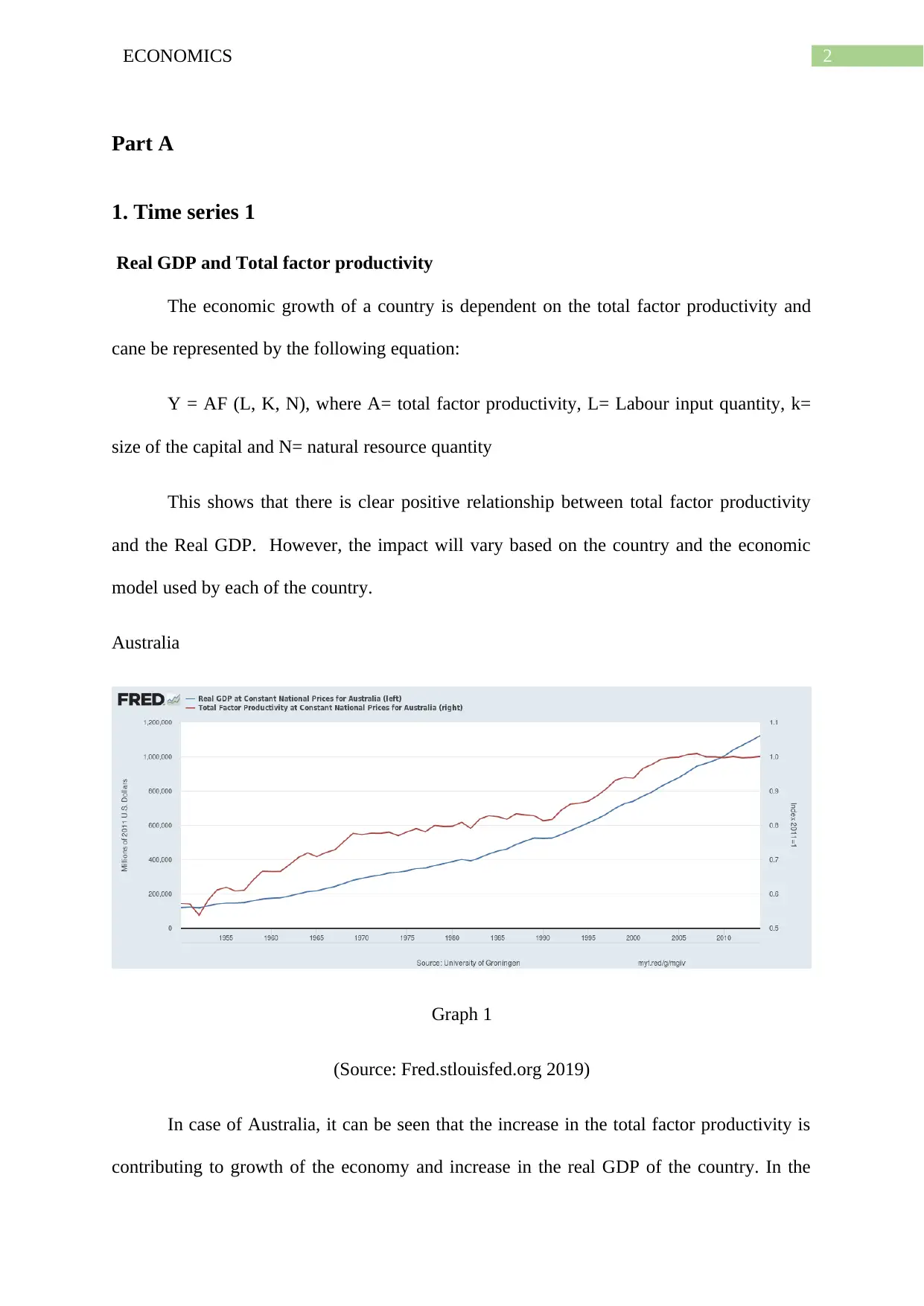
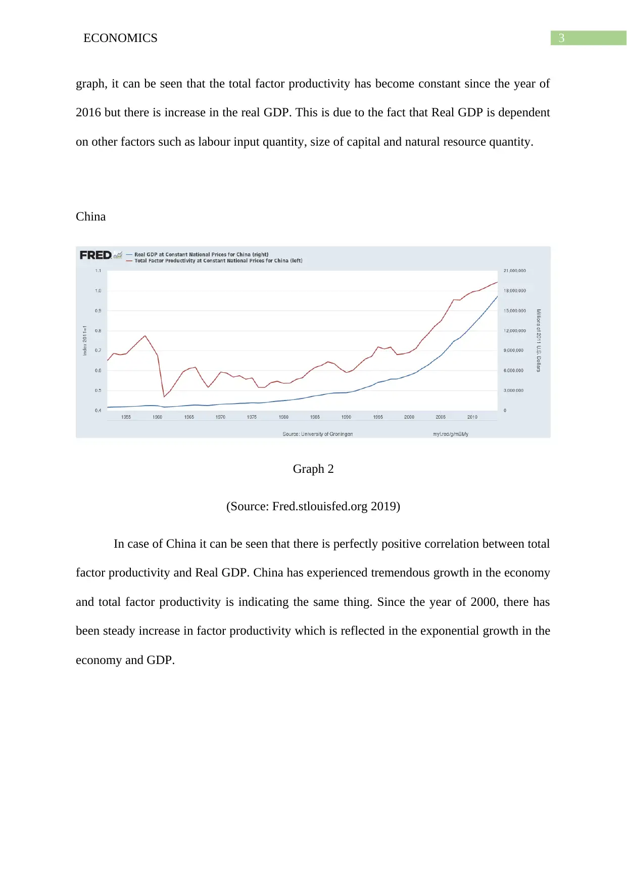
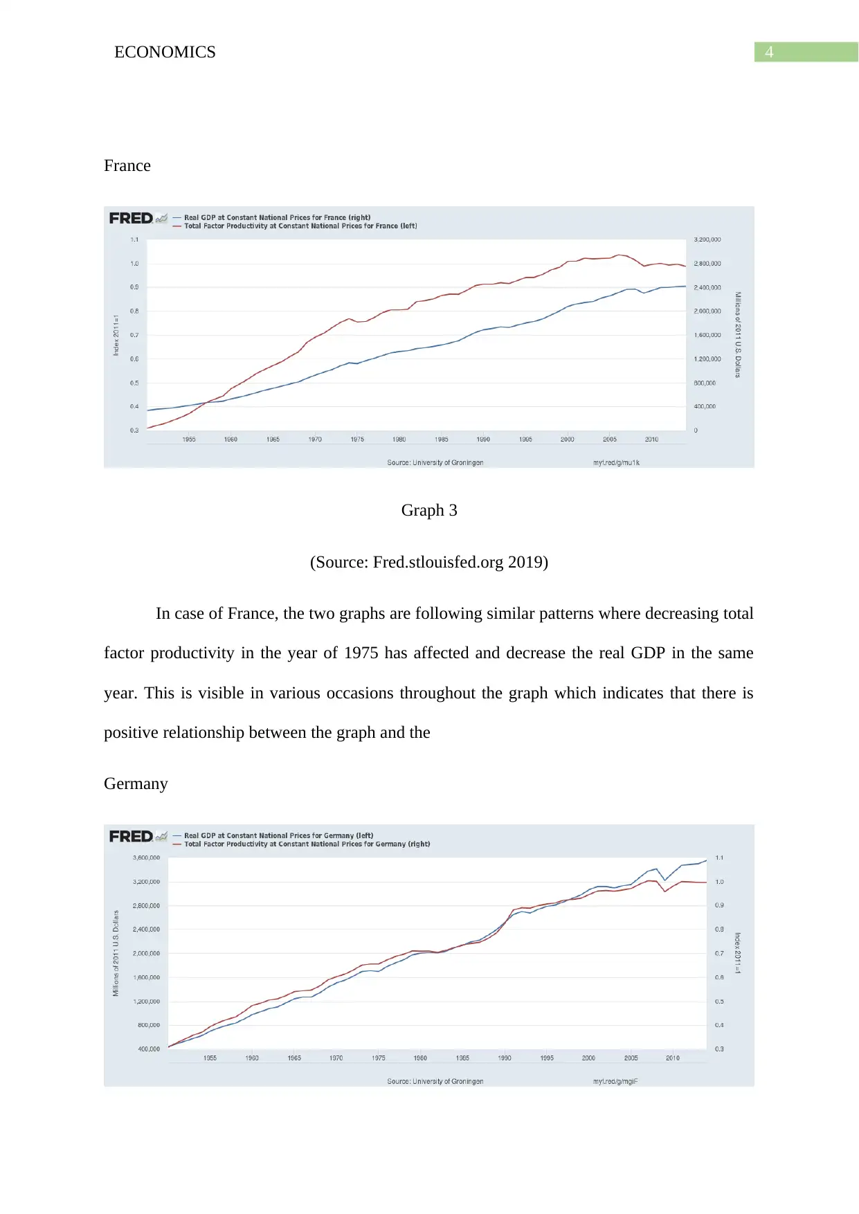
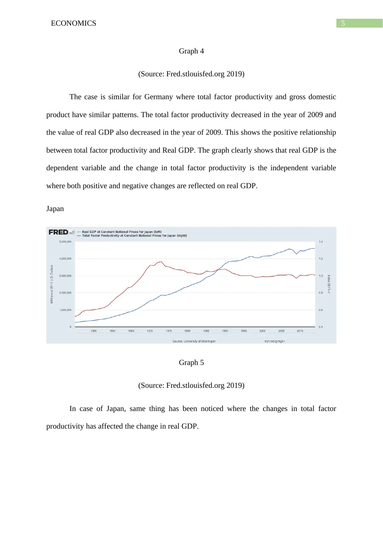
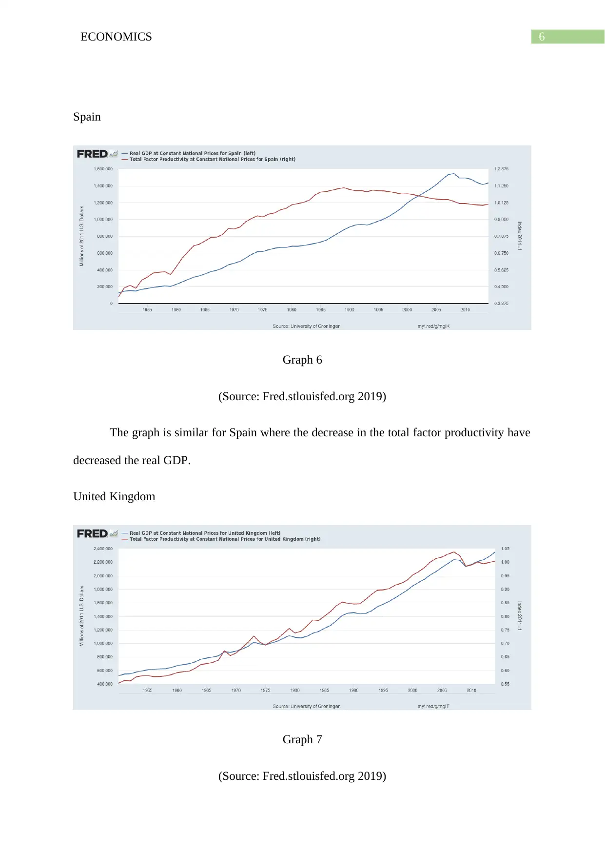
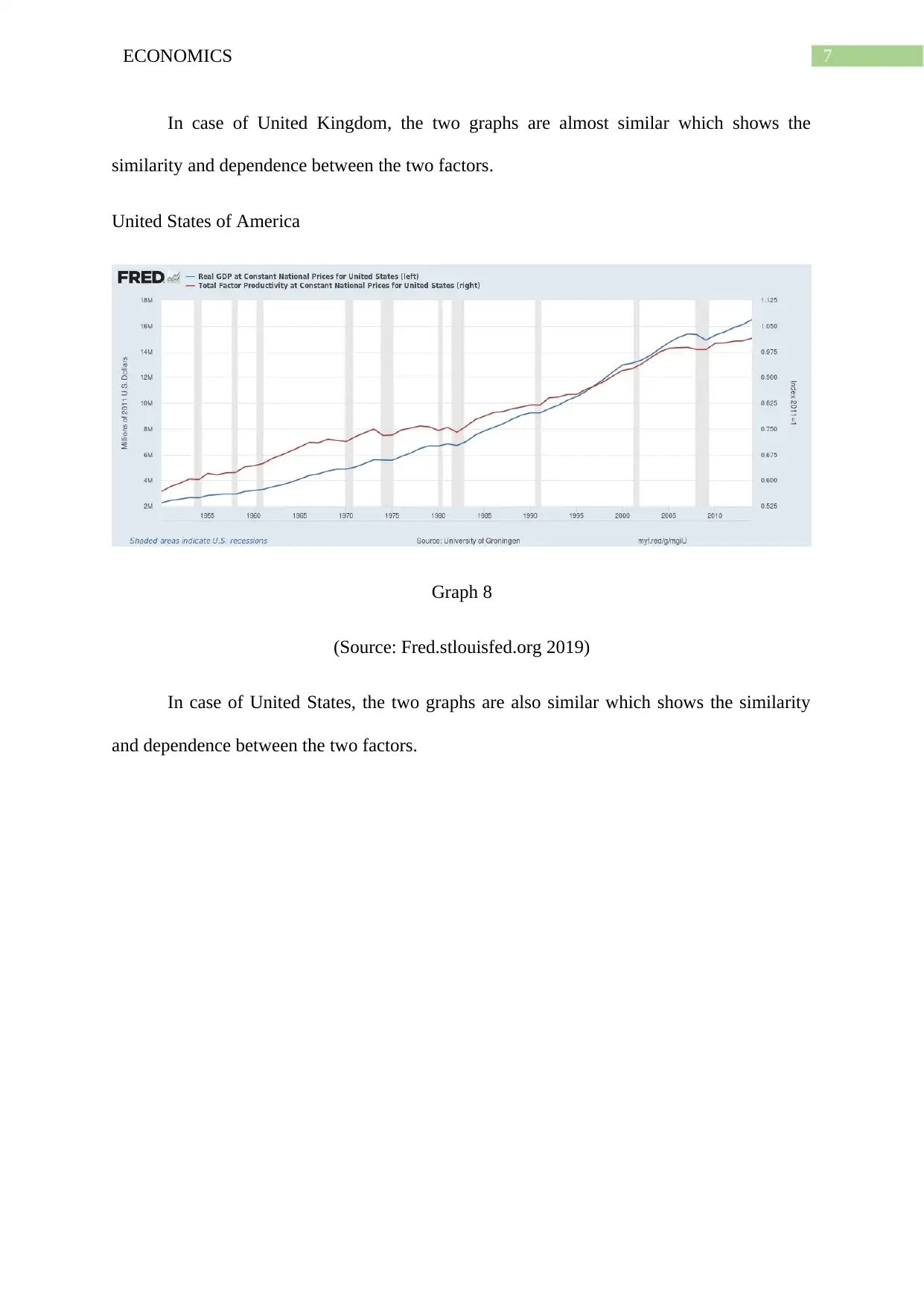
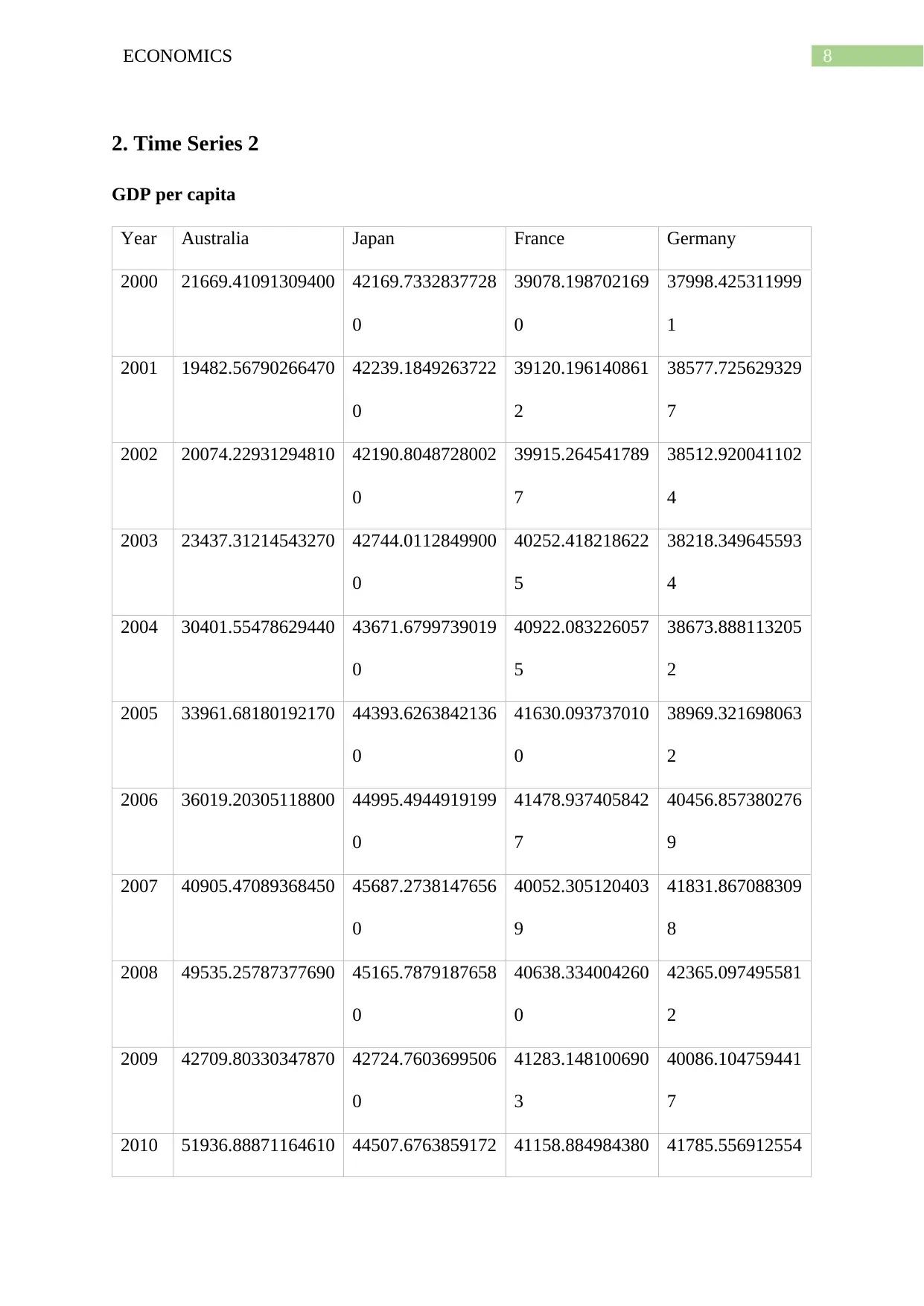
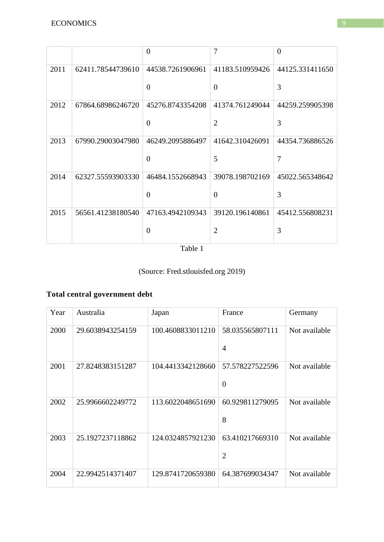
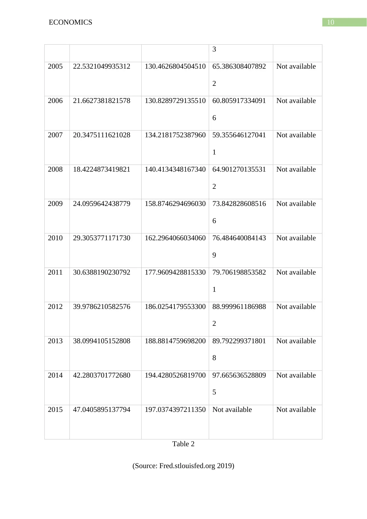
This economics report provides a detailed analysis of key economic indicators including Real GDP, total factor productivity, GDP per capita, government debt, imports, government final consumption expenditure, and job vacancies, focusing primarily on Australia and making comparisons with other countries like China, France, Germany, Japan, Spain, the United Kingdom, and the United States. It examines the relationship between total factor productivity and Real GDP, highlighting the positive correlation across various economies. The report also explores the impact of government expenditure on GDP in both the short and long run, using aggregate demand and supply curves to illustrate the effects on real GDP and prices. Furthermore, it investigates the inverse relationship between unemployment rates and job vacancies in Australia. The report concludes with a discussion of potential career paths for economics graduates, focusing on the role of a data scientist within the Department of Premier & Cabinet and emphasizing the importance of analytical and communication skills. Desklib offers this and many other solved assignments to help students.

Running head: ECONOMICS
Economics
Name of the student
Name of the university
Author note

1ECONOMICS
Table of Contents
Part A.........................................................................................................................................2
1. Time series 1..........................................................................................................................2
Real GDP and Total factor productivity................................................................................2
2. Time Series 2..........................................................................................................................8
GDP per capita.......................................................................................................................8
Total central government debt.............................................................................................9
Imports: Value Goods..........................................................................................................11
Government Final Consumption Expenditure.....................................................................12
Relationship between GDP and government final consumption expenditure.....................14
3. Time series 3........................................................................................................................15
Total Unfilled Job Vacancies for Australia vs Unemployment rate....................................15
Part B........................................................................................................................................16
Part C........................................................................................................................................18
References................................................................................................................................20
Appendix..................................................................................................................................22

2ECONOMICS
Part A
1. Time series 1
Real GDP and Total factor productivity
The economic growth of a country is dependent on the total factor productivity and
cane be represented by the following equation:
Y = AF (L, K, N), where A= total factor productivity, L= Labour input quantity, k=
size of the capital and N= natural resource quantity
This shows that there is clear positive relationship between total factor productivity
and the Real GDP. However, the impact will vary based on the country and the economic
model used by each of the country.
Australia
Graph 1
(Source: Fred.stlouisfed.org 2019)
In case of Australia, it can be seen that the increase in the total factor productivity is
contributing to growth of the economy and increase in the real GDP of the country. In the

3ECONOMICS
graph, it can be seen that the total factor productivity has become constant since the year of
2016 but there is increase in the real GDP. This is due to the fact that Real GDP is dependent
on other factors such as labour input quantity, size of capital and natural resource quantity.
China
Graph 2
(Source: Fred.stlouisfed.org 2019)
In case of China it can be seen that there is perfectly positive correlation between total
factor productivity and Real GDP. China has experienced tremendous growth in the economy
and total factor productivity is indicating the same thing. Since the year of 2000, there has
been steady increase in factor productivity which is reflected in the exponential growth in the
economy and GDP.

4ECONOMICS
France
Graph 3
(Source: Fred.stlouisfed.org 2019)
In case of France, the two graphs are following similar patterns where decreasing total
factor productivity in the year of 1975 has affected and decrease the real GDP in the same
year. This is visible in various occasions throughout the graph which indicates that there is
positive relationship between the graph and the
Germany

5ECONOMICS
Graph 4
(Source: Fred.stlouisfed.org 2019)
The case is similar for Germany where total factor productivity and gross domestic
product have similar patterns. The total factor productivity decreased in the year of 2009 and
the value of real GDP also decreased in the year of 2009. This shows the positive relationship
between total factor productivity and Real GDP. The graph clearly shows that real GDP is the
dependent variable and the change in total factor productivity is the independent variable
where both positive and negative changes are reflected on real GDP.
Japan
Graph 5
(Source: Fred.stlouisfed.org 2019)
In case of Japan, same thing has been noticed where the changes in total factor
productivity has affected the change in real GDP.

6ECONOMICS
Spain
Graph 6
(Source: Fred.stlouisfed.org 2019)
The graph is similar for Spain where the decrease in the total factor productivity have
decreased the real GDP.
United Kingdom
Graph 7
(Source: Fred.stlouisfed.org 2019)

7ECONOMICS
In case of United Kingdom, the two graphs are almost similar which shows the
similarity and dependence between the two factors.
United States of America
Graph 8
(Source: Fred.stlouisfed.org 2019)
In case of United States, the two graphs are also similar which shows the similarity
and dependence between the two factors.

8ECONOMICS
2. Time Series 2
GDP per capita
Year Australia Japan France Germany
2000 21669.41091309400 42169.7332837728
0
39078.198702169
0
37998.425311999
1
2001 19482.56790266470 42239.1849263722
0
39120.196140861
2
38577.725629329
7
2002 20074.22931294810 42190.8048728002
0
39915.264541789
7
38512.920041102
4
2003 23437.31214543270 42744.0112849900
0
40252.418218622
5
38218.349645593
4
2004 30401.55478629440 43671.6799739019
0
40922.083226057
5
38673.888113205
2
2005 33961.68180192170 44393.6263842136
0
41630.093737010
0
38969.321698063
2
2006 36019.20305118800 44995.4944919199
0
41478.937405842
7
40456.857380276
9
2007 40905.47089368450 45687.2738147656
0
40052.305120403
9
41831.867088309
8
2008 49535.25787377690 45165.7879187658
0
40638.334004260
0
42365.097495581
2
2009 42709.80330347870 42724.7603699506
0
41283.148100690
3
40086.104759441
7
2010 51936.88871164610 44507.6763859172 41158.884984380 41785.556912554

9ECONOMICS
0 7 0
2011 62411.78544739610 44538.7261906961
0
41183.510959426
0
44125.331411650
3
2012 67864.68986246720 45276.8743354208
0
41374.761249044
2
44259.259905398
3
2013 67990.29003047980 46249.2095886497
0
41642.310426091
5
44354.736886526
7
2014 62327.55593903330 46484.1552668943
0
39078.198702169
0
45022.565348642
3
2015 56561.41238180540 47163.4942109343
0
39120.196140861
2
45412.556808231
3
Table 1
(Source: Fred.stlouisfed.org 2019)
Total central government debt
Year Australia Japan France Germany
2000 29.6038943254159 100.4608833011210 58.035565807111
4
Not available
2001 27.8248383151287 104.4413342128660 57.578227522596
0
Not available
2002 25.9966602249772 113.6022048651690 60.929811279095
8
Not available
2003 25.1927237118862 124.0324857921230 63.410217669310
2
Not available
2004 22.9942514371407 129.8741720659380 64.387699034347 Not available

10ECONOMICS
3
2005 22.5321049935312 130.4626804504510 65.386308407892
2
Not available
2006 21.6627381821578 130.8289729135510 60.805917334091
6
Not available
2007 20.3475111621028 134.2181752387960 59.355646127041
1
Not available
2008 18.4224873419821 140.4134348167340 64.901270135531
2
Not available
2009 24.0959642438779 158.8746294696030 73.842828608516
6
Not available
2010 29.3053771171730 162.2964066034060 76.484640084143
9
Not available
2011 30.6388190230792 177.9609428815330 79.706198853582
1
Not available
2012 39.9786210582576 186.0254179553300 88.999961186988
2
Not available
2013 38.0994105152808 188.8814759698200 89.792299371801
8
Not available
2014 42.2803701772680 194.4280526819700 97.665636528809
5
Not available
2015 47.0405895137794 197.0374397211350 Not available Not available
Table 2
(Source: Fred.stlouisfed.org 2019)

11ECONOMICS
Data for Germany only available from 1990 to 1998
1990-01-01 21.0100829162179
1991-01-01 22.0359098082079
1992-01-01 24.1833109888399
1993-01-01 26.3960592533607
1994-01-01 28.0509505326032
1995-01-01 35.1974848331648
1996-01-01 36.4464540546626
1997-01-01 37.0312259805221
1998-01-01 37.0345432564334
Table 3
(Source: Fred.stlouisfed.org 2019)
Imports: Value Goods
Year Australia Japan France Germany
200
0
17.044323195794
20
379978562482.2060
00
338846280239.0150
00
25.34163994972
01
200
1
16.163159703097
20
349063604269.4810
00
329067896994.0550
00
24.86532651983
45
200
2
16.347893452510
90
337670852451.9140
00
330168706911.5950
00
23.42073210855
29

12ECONOMICS
200
3
15.740239891363
30
383042031877.8280
00
399263496612.7790
00
24.02308309975
35
200
4
15.741006126759
10
453729619054.9230
00
467004809724.6100
00
25.22133866664
21
200
5
16.233783000937
60
518761532102.5360
00
502468116187.4910
00
26.98467273478
32
200
6
17.056841378176
20
578829472888.5740
00
543762449815.3030
00
30.07785024854
52
200
7
16.627011134988
80
624018129628.6840
00
632238722107.5780
00
30.60930691472
90
200
8
18.205542109884
90
763081577471.6790
00
715033586928.1110
00
31.41017329939
47
200
9
15.923597607223
00
551396426302.2210
00
563431343906.9040
00
26.92447142863
78
201
0
15.464289163324
70
694497155354.1560
00
607373910028.9110
00
30.67465107775
66
201
1
15.492002287516
10
858342674597.3120
00
718571195289.7890
00
33.17739316756
84
201
2
15.994830815877
40
883288393273.5560
00
674590744046.5470
00
32.56430761777
82
201
3
15.362495628424
00
831821139901.4390
00
684543992500.1700
00
31.41826176385
23
201
4
15.676716740580
50
812266004467.7150
00
681155420924.3860
00
30.85673503380
28
201 16.275064168219 648151124839.4600 574727552031.9870 30.96653767428

13ECONOMICS
5 10 00 00 17
Table 4
(Source: Fred.stlouisfed.org 2019)
Government Final Consumption Expenditure
Year Australia Japan France Germany
2000 200580000000.0000
0
83899400000000 41852400000
0
437798700000.0000
0
2001 204860000000.0000
0
86760000000000 42285400000
0
440043370000.0000
0
2002 208934000000.0000
0
89061900000000 43046200000
0
445334410000.0000
0
2003 219511000000.0000
0
90709000000000 43877800000
0
447776420000.0000
0
2004 227255000000.0000
0
91776100000000 44834900000
0
444224410000.0000
0
2005 234178000000.0000
0
92505000000000 45401100000
0
446370420000.0000
0
2006 242452000000.0000
0
92567200000000 46010800000
0
450674760000.0000
0
2007 248355000000.0000
0
93635500000000 46847200000
0
457273140000.0000
0
2008 258692000000.0000
0
93561600000000 47379600000
0
472788560000.0000
0
2009 264920000000.0000 95472300000000 48520700000 487021300000.0000

14ECONOMICS
0 0 0
2010 271855000000.0000
0
97323800000000 49142000000
0
493336000000.0000
0
2011 283507000000.0000
0
99204600000000 49659200000
0
497961020000.0000
0
2012 287703000000.0000
0
10086900000000
0
50453200000
0
503202730000.0000
0
2013 291900000000.0000
0
10238220000000
0
51196700000
0
510010760000.0000
0
2014 293823000000.0000
0
10293760000000
0
51865000000
0
517965810000.0000
0
2015 305274000000.0000
0
10452400000000
0
52386900000
0
533160550000.0000
0
Table 5
(Source: Fred.stlouisfed.org 2019)
Relationship between GDP and government final consumption expenditure
Gross domestic product can be represented by the formula,
PIB = CF + I + G + (X – M), where
CF= household final consumption expenditure,
I= Investment,
X= government expenditures,
M= export value and I = import value

15ECONOMICS
The data collected shows the similar relationship where it can be seen that there is
increasing in GDP with increase in government final consumption expenditure. Government
final consumption expenditure highlights the movement of income and contribution of the
government to the economy. The tables reflect that with increase in the government final
consumption expenditure, there has been increase in the gross domestic product of the all the
given countries.
3. Time series 3
Total Unfilled Job Vacancies for Australia vs Unemployment rate
Graph 9
(Source: Fred.stlouisfed.org 2019)
The graph clearly depicts an inversely proportional relationship between
unemployment rate and total unfilled job vacancies. There is negative correlation between
both the variables where increase in the total unfilled vacancy means that there will be
decrease in the unemployment rate. High unfilled job vacancies shows that the demand of
talent is high in the market and there will be decrease in the unemployment rate. The graph

16ECONOMICS
shows that in recent years, there has been significant increase in demand of talents and
decrease in unemployment rate in the country.

17ECONOMICS
Part B
Short run effect with increase in government expenditure
Graph 10
Source: (2012books.lardbucket.org 2019)
In state of equilibrium where P1=Y1 , the increase in government expenditure will
move the aggregate demand supply curve outwards. Government expenditure is one of the
key components of aggregate demand and increase in the government expenditure will shift
the short run curve from Y1 to Y2 (Gemmell, Kneller and Sanz 2016). The shift in equilibrium
position from P1 to P2 shows that there will be increase real GDP and prices. This means that
the economy is booming and there will be significant decrease in the unemployment rate in
the country.

18ECONOMICS
Long run effect with increase in government expenditure
Graph 11
Source: (2012books.lardbucket.org 2019)
The impact of increase in aggregate demand depends on the economic
situation of a country. The increase in tax amount will not cause any change to the aggregate
demand. The increase in the government spending may increase in the overall GDP of the
country. The increase in government spending causes a multiplier effect. Suppose the
government expenditure decreases the unemployment rate, then there will be increase in the
aggregate demand (Dunne 2015). The graph shows that there has been outward movement of
long run curve which shows that there is increase in demand and supply at the same time.
This will increase in working population and productivity of the labours. There will be no
change to the price level but there will be significant increase in supply, demand and GDP of
the country.

19ECONOMICS

20ECONOMICS
Part C
The organization I have chosen to work with is Department of Premier & Cabinet.
This department belongs to the government of Victorian State. The department deals with the
economic policies, state productivity, social policy, public sector ICT, service delivery
reforms, and digital government, office of multicultural affairs and Citizenship and office of
Aboriginal Affairs.
The company has recently advertised for a job of a Data Scientist which is one of the
primary roles that I want to take up to after completing my degree in the field of economics.
My main role will be dealing with data of different types that would analyse and forecast
future economic policies, productivity of the state, social policies and other reforms. My main
role is collecting and analysing to data to understand the position of the economy and help the
government develop effective economic and other policies for improving the productivity of
the state and the overall GDP of the country. I will be able to implement all the learnings
from the Economics Learning Standards for Bachelor graduate students. I have made
significant efforts in improving my communication and organizational skills but there are
many aspect where I am still lagging experience. I have gained theoretical knowledge about
all the topics in economies but I need better understanding of the practical implications and
the way analytical skills can be put to use effectively to understand the impact of different
factors on the economic growth. I will strive to make effort so that I can gain knowledge
about concepts taught in Economics Learning Standards for Bachelor graduate students, more
adequately. I want to show my capabilities to different recruiters in present and future times
where I would like to display the knowledge gained through portfolios, extracurricular
activities and university learnings.

21ECONOMICS
I have always been good in numbers and have experienced great satisfaction in
quantitative studies. The job of a Data Scientist is one of the ideal jobs for me as I have ways
wanted to work on data to develop new findings about the economy and contribute to
Australia in some way. My personality tests suggests that I am an innovator which means that
I am best suited to the jobs that are technical, scientific and have practical implications to it. I
am thoughtful, analytical and logical by nature which will help me in solve issues. I prefer
making decisions based on data and data scientist is one of the suitable jobs for me.
The economic informational interview showed that economics can be used to explain
the way the whole global economy is working and how it can be used effectively to
contribute and make changes to the world policies for sustinable and better future. The
interview suggested us to use economic theories during the internship so that will increase
our practical knowldege regarding the application of economics. This is the reason I have
chosen the job of a Data Scientist as I will be able to contribute to new policy formulation
and contribute to the economic growth of the country in the smallest possible way. I want to
work towards something that would contribute to the society as illustrated in the interview.
I have understood there are many things I still need to learn to reach a level of
excellence in my chosen field. I want to increase my level of analytical skills and application
of theories to understand the way the different factors in economy play a part in the wellbeing
of the society. I want to gain more knowledge on conducting research of different types and
be part of different research programs to understand the economic concepts in a better way
and improve my skill level.

22ECONOMICS
References
2012books.lardbucket.org 2019. Aggregate Demand and Aggregate Supply: The Long Run
and the Short Run. [online] 2012books.lardbucket.org. Available at:
https://2012books.lardbucket.org/books/macroeconomics-principles-v1.1/s10-02-aggregate-
demand-and-aggregate.html [Accessed 14 Jan. 2019].
Dunne, J.P., 2015. Economic effects of military expenditure in developing countries.
Fred.stlouisfed.org 2019. Real GDP at Constant National Prices for Australia. [online]
Fred.stlouisfed.org. Available at:
https://fred.stlouisfed.org/series/RGDPNAAUA666NRUG#0 [Accessed 14 Jan. 2019].
Fred.stlouisfed.org 2019. Real GDP at Constant National Prices for China. [online]
Fred.stlouisfed.org. Available at:
https://fred.stlouisfed.org/series/RGDPNACNA666NRUG#0 [Accessed 14 Jan. 2019].
Fred.stlouisfed.org 2019. Real GDP at Constant National Prices for Germany. [online]
Fred.stlouisfed.org. Available at:
https://fred.stlouisfed.org/series/RGDPNADEA666NRUG#0 [Accessed 14 Jan. 2019].
Fred.stlouisfed.org 2019. Real GDP at Constant National Prices for United States. [online]
Fred.stlouisfed.org. Available at:
https://fred.stlouisfed.org/series/RGDPNAUSA666NRUG#0 [Accessed 14 Jan. 2019].
Fred.stlouisfed.org 2019. Real GDP at Constant National Prices for United Kingdom.
[online] Fred.stlouisfed.org. Available at:
https://fred.stlouisfed.org/series/RGDPNAGBA666NRUG#0 [Accessed 14 Jan. 2019].

23ECONOMICS
Fred.stlouisfed.org 2019. Real GDP at Constant National Prices for Spain. [online]
Fred.stlouisfed.org. Available at:
https://fred.stlouisfed.org/series/RGDPNAESA666NRUG#0 [Accessed 14 Jan. 2019].
Fred.stlouisfed.org 2019. Real GDP at Constant National Prices for Japan. [online]
Fred.stlouisfed.org. Available at: https://fred.stlouisfed.org/series/RGDPNAJPA666NRUG#0
[Accessed 14 Jan. 2019].
Gemmell, N., Kneller, R. and Sanz, I., 2016. Does the Composition of Government
Expenditure Matter for Long‐Run GDP Levels?. Oxford Bulletin of Economics and
Statistics, 78(4), pp.522-547.

24ECONOMICS
Appendix