Analyzing Ozone Layer Trends: A Time Series Regression Approach

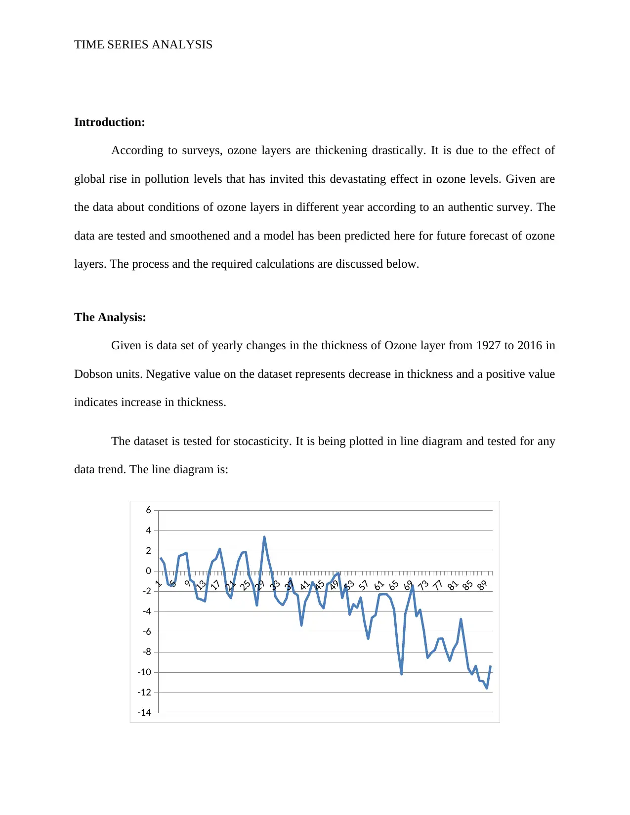
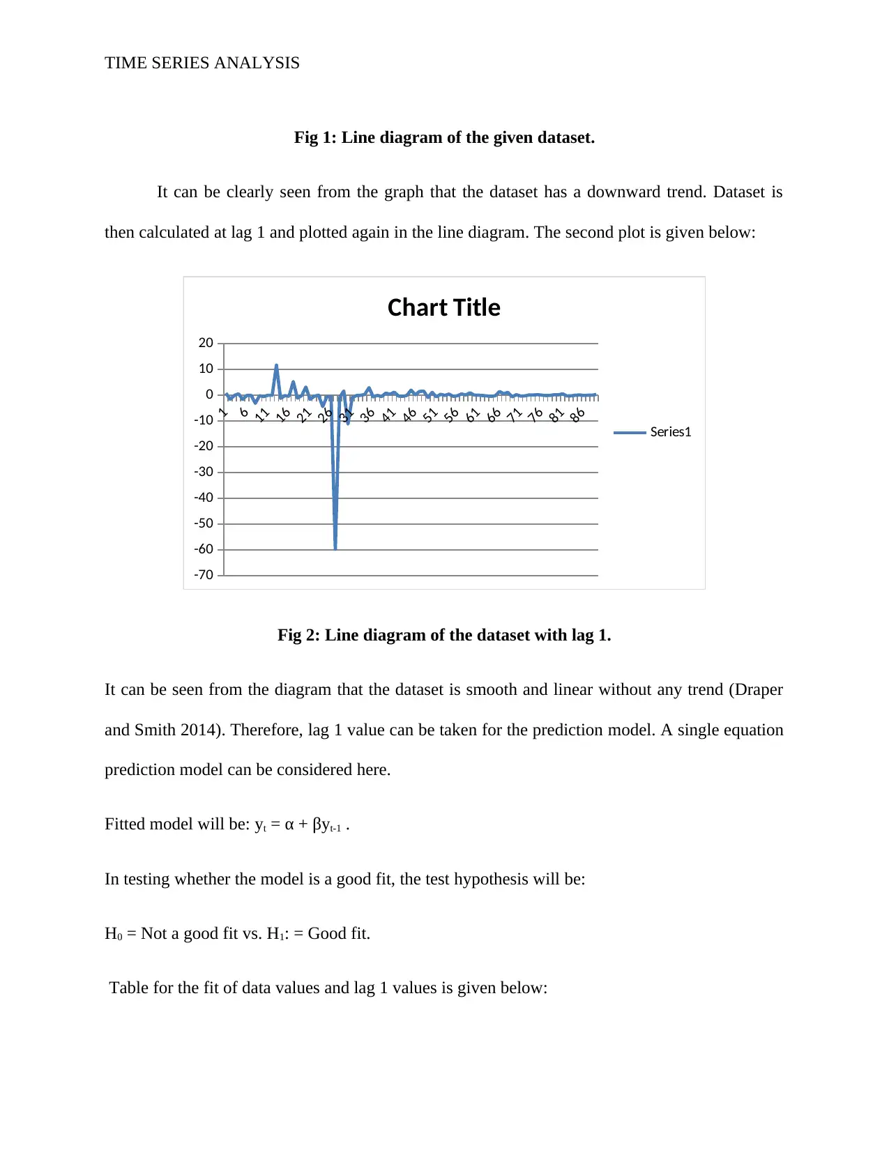
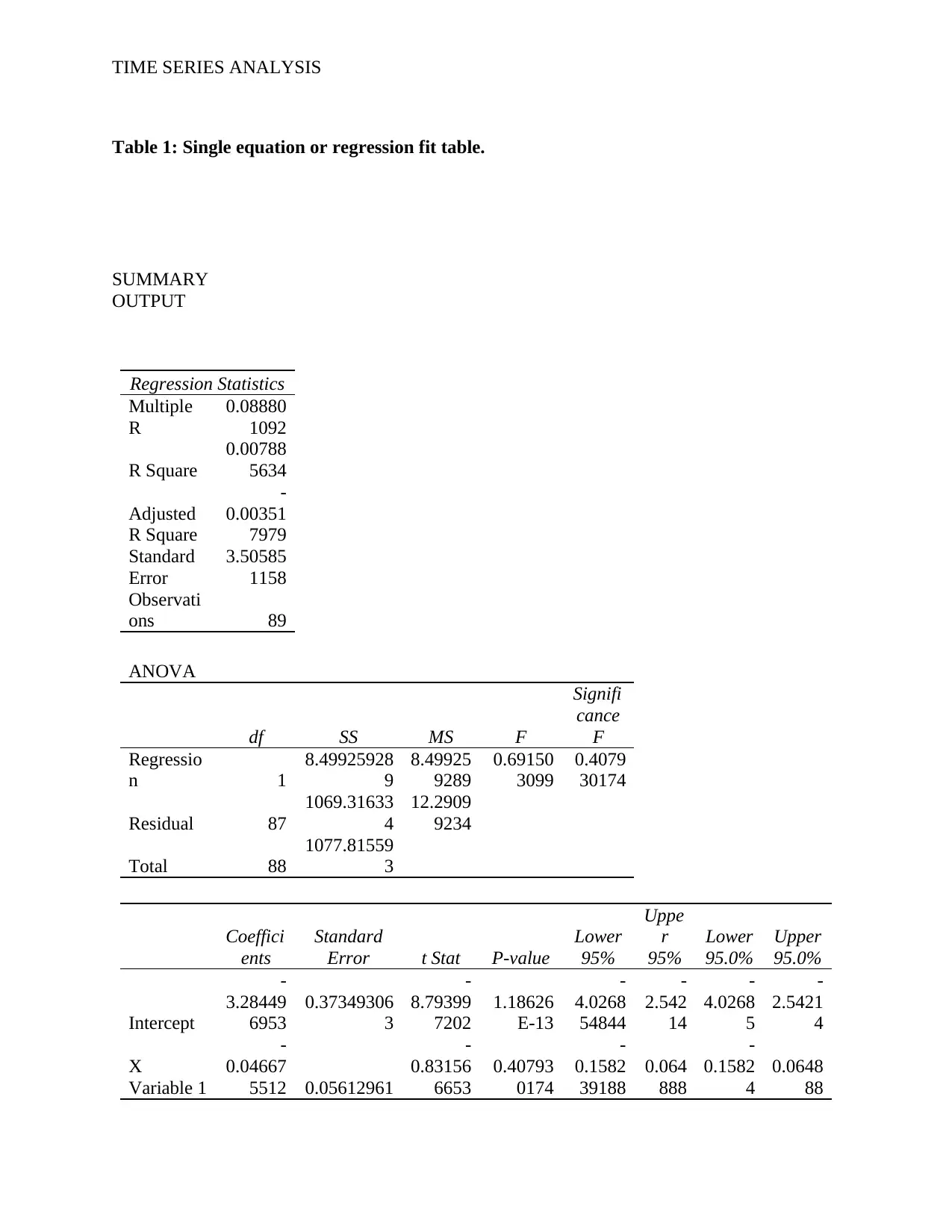
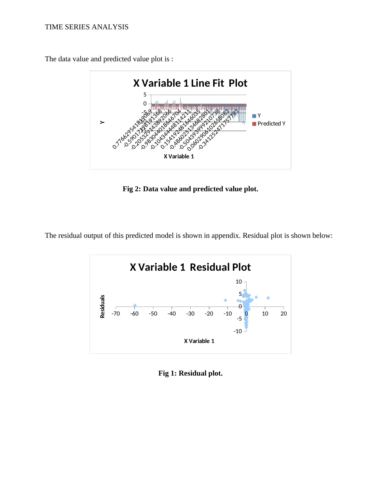
This report presents a time series analysis of ozone layer thickness data from 1927 to 2016, measured in Dobson units. The analysis identifies a downward trend in the initial data, which is subsequently smoothed. A regression model is fitted to the data, and ANOVA and P-value tests confirm that the model is a good fit for forecasting future ozone levels. The model, represented as yt = (-0.046)yt-1, relates current ozone levels to those at lag 1. Residual and predicted value plots are included to visualize the model's performance. The report concludes that this model can be used to predict future ozone levels based on past trends, providing valuable insights for environmental monitoring and policy-making. Desklib provides access to this and other solved assignments.

Running head: TIME SERIES ANALYSIS
TIME SERIES ANALYSIS
Name of the student:
Name of the university:
Author’s note:

TIME SERIES ANALYSIS
Executive summary
Ozone layers are thickening drastically now a days which has raised an alarming situation. The
reason is considered as global raise in pollution levels. Data are given about the condition of
ozone layers. A model has been fitted here for predicting ozone levels in the future.

TIME SERIES ANALYSIS
Table of Contents
Introduction:....................................................................................................................................3
The Analysis:...................................................................................................................................3
Conclusion:......................................................................................................................................3
References:......................................................................................................................................4
Appendix:........................................................................................................................................5

TIME SERIES ANALYSIS
Introduction:
According to surveys, ozone layers are thickening drastically. It is due to the effect of
global rise in pollution levels that has invited this devastating effect in ozone levels. Given are
the data about conditions of ozone layers in different year according to an authentic survey. The
data are tested and smoothened and a model has been predicted here for future forecast of ozone
layers. The process and the required calculations are discussed below.
The Analysis:
Given is data set of yearly changes in the thickness of Ozone layer from 1927 to 2016 in
Dobson units. Negative value on the dataset represents decrease in thickness and a positive value
indicates increase in thickness.
The dataset is tested for stocasticity. It is being plotted in line diagram and tested for any
data trend. The line diagram is:
1
5
9
13
17
21
25
29
33
37
41
45
49
53
57
61
65
69
73
77
81
85
89
-14
-12
-10
-8
-6
-4
-2
0
2
4
6

TIME SERIES ANALYSIS
Fig 1: Line diagram of the given dataset.
It can be clearly seen from the graph that the dataset has a downward trend. Dataset is
then calculated at lag 1 and plotted again in the line diagram. The second plot is given below:
1
6
11
16
21
26
31
36
41
46
51
56
61
66
71
76
81
86
-70
-60
-50
-40
-30
-20
-10
0
10
20
Chart Title
Series1
Fig 2: Line diagram of the dataset with lag 1.
It can be seen from the diagram that the dataset is smooth and linear without any trend (Draper
and Smith 2014). Therefore, lag 1 value can be taken for the prediction model. A single equation
prediction model can be considered here.
Fitted model will be: yt = α + βyt-1 .
In testing whether the model is a good fit, the test hypothesis will be:
H0 = Not a good fit vs. H1: = Good fit.
Table for the fit of data values and lag 1 values is given below:

TIME SERIES ANALYSIS
Table 1: Single equation or regression fit table.
SUMMARY
OUTPUT
Regression Statistics
Multiple
R
0.08880
1092
R Square
0.00788
5634
Adjusted
R Square
-
0.00351
7979
Standard
Error
3.50585
1158
Observati
ons 89
ANOVA
df SS MS F
Signifi
cance
F
Regressio
n 1
8.49925928
9
8.49925
9289
0.69150
3099
0.4079
30174
Residual 87
1069.31633
4
12.2909
9234
Total 88
1077.81559
3
Coeffici
ents
Standard
Error t Stat P-value
Lower
95%
Uppe
r
95%
Lower
95.0%
Upper
95.0%
Intercept
-
3.28449
6953
0.37349306
3
-
8.79399
7202
1.18626
E-13
-
4.0268
54844
-
2.542
14
-
4.0268
5
-
2.5421
4
X
Variable 1
-
0.04667
5512 0.05612961
-
0.83156
6653
0.40793
0174
-
0.1582
39188
0.064
888
-
0.1582
4
0.0648
88

TIME SERIES ANALYSIS
It can be said from the table that required prediction model is yt = (-0.046)yt-1, where yt are the
given data values and yt-1 are the values at lag 1. F – statistic for ANOVA test is 0.691 and
tabulated F at 5% level of significance is 0.407. F – statistic > Tabulated F. Therefore, the null
hypothesis will be rejected here at 5% level of significance and the model is a good fit (Bennell
and Canter 2017). Again, P-value of the intercept is 1.18626E-13 which is less than 0.05 and
therefore intercept term can be rejected. P – value of Variable 1 is 0.4079 and hence, variable 1
can be accepted.

TIME SERIES ANALYSIS
The data value and predicted value plot is :
0.776629541819069
-0.59017198191368
-0.205329143892066
-0.983044018646704
-0.104344448114211
0.154192481646035
-0.486025134682801
-0.504393999210738
0.0602906102658083
-0.341252471757783
-15
-10
-5
0
5
X Variable 1 Line Fit Plot
Y
Predicted Y
X Variable 1
Y
Fig 2: Data value and predicted value plot.
The residual output of this predicted model is shown in appendix. Residual plot is shown below:
-70 -60 -50 -40 -30 -20 -10 0 10 20
-10
-5
0
5
10
X Variable 1 Residual Plot
X Variable 1
Residuals
Fig 1: Residual plot.

TIME SERIES ANALYSIS
Conclusion:
Data for different years are being calculated and smoothened and tabulated. The data
shows a downward trend initially which is smoothened. A regression line is being fitted here
which is a good fit for the dataset according to the test results. Therefore, future value of the
ozone levels can be calculated through this fit.

TIME SERIES ANALYSIS
References:
Bennell, C. and Canter, D.V., 2017. „Linking Commercial Burglaries by Modus Operandi: Tests
Using Regression and ROC Analysis‟. Science and Justice.
Draper, N.R. and Smith, H., 2014. Applied regression analysis(Vol. 326). John Wiley & Sons.

TIME SERIES ANALYSIS
Appendix:
Predicted values, Residual values and standard residual values:
RESIDUAL
OUTPUT
Observation Predicted Y Residuals
Standard
Residuals
1
-
3.320746535 4.08127895 1.170804856
2
-
3.209838284 1.941280938 0.556899241
3
-
3.278274459 1.814587285 0.520554373
4
-
3.307590781 2.328387759 0.667949368
5
-
3.207524618 4.71609208 1.352914999
6
-
3.281021903 4.910938711 1.408811052
7
-
3.279338704 5.111762035 1.46642165
8
-
3.135962487 2.296278847 0.658738218
9
-
3.273577398 2.177461738 0.624652911
10
-
3.256950374 0.582375646 0.167067295
11
-
3.282611433 0.495445373 0.142129429
12
-
3.281576756 0.308397314 0.08847057
13
-
3.828463862 3.593508383 1.030877114
14
-
3.226523403 4.197193407 1.204057473
15
-
3.274461695 4.510984766 1.294075444
16
-
3.263695531 5.494318843 1.576166505
17
-
3.529693344 3.886409713 1.114902318

TIME SERIES ANALYSIS
18
-
3.229968747 1.109687755 0.3183384
19 -3.27491311 0.606788344 0.174070616
20 -3.43029549 2.783267538 0.798441662
21
-
3.207502401 4.203588041 1.205891915
22
-
3.263114325 5.101291748 1.463418017
23
-
3.282996596 5.182223571 1.486635095
24
-
3.078062216 2.52318101 0.723830107
25
-
3.256269935 1.85239574 0.531400562
26
-
3.257140619 -0.134647004 -0.038626462
27
-
0.497504628 0.55527657 0.159293327
28 -3.23861287 6.645784699 1.906489875
29
-
3.358768624 4.673652415 1.340740245
30
-
2.761414836 2.63259027 0.755216565
31
-
3.240211516 0.724410151 0.207813024
32 -3.27617028 0.214113637 0.061423218
33
-
3.280659311 -0.055712483 -0.015982354
34
-
3.296292352 0.63297037 0.181581507
35
-
3.420744303 2.741157748 0.78636154
36
-
3.252807734 1.136203519 0.325945032
37
-
3.279626623 0.916436655 0.262900061
38 -3.25839437 -2.103171005 -0.603340976
39
-
3.320385267 0.289350689 0.083006625
40
-
3.299644524 1.011258282 0.290101736
41
-
3.338171799 2.273784964 0.652285352
42
-
3.267250829 1.579115128 0.453003993