Statistical Analysis Case Study: Graduation Rates and Study Time
VerifiedAdded on 2020/04/13
|6
|765
|470
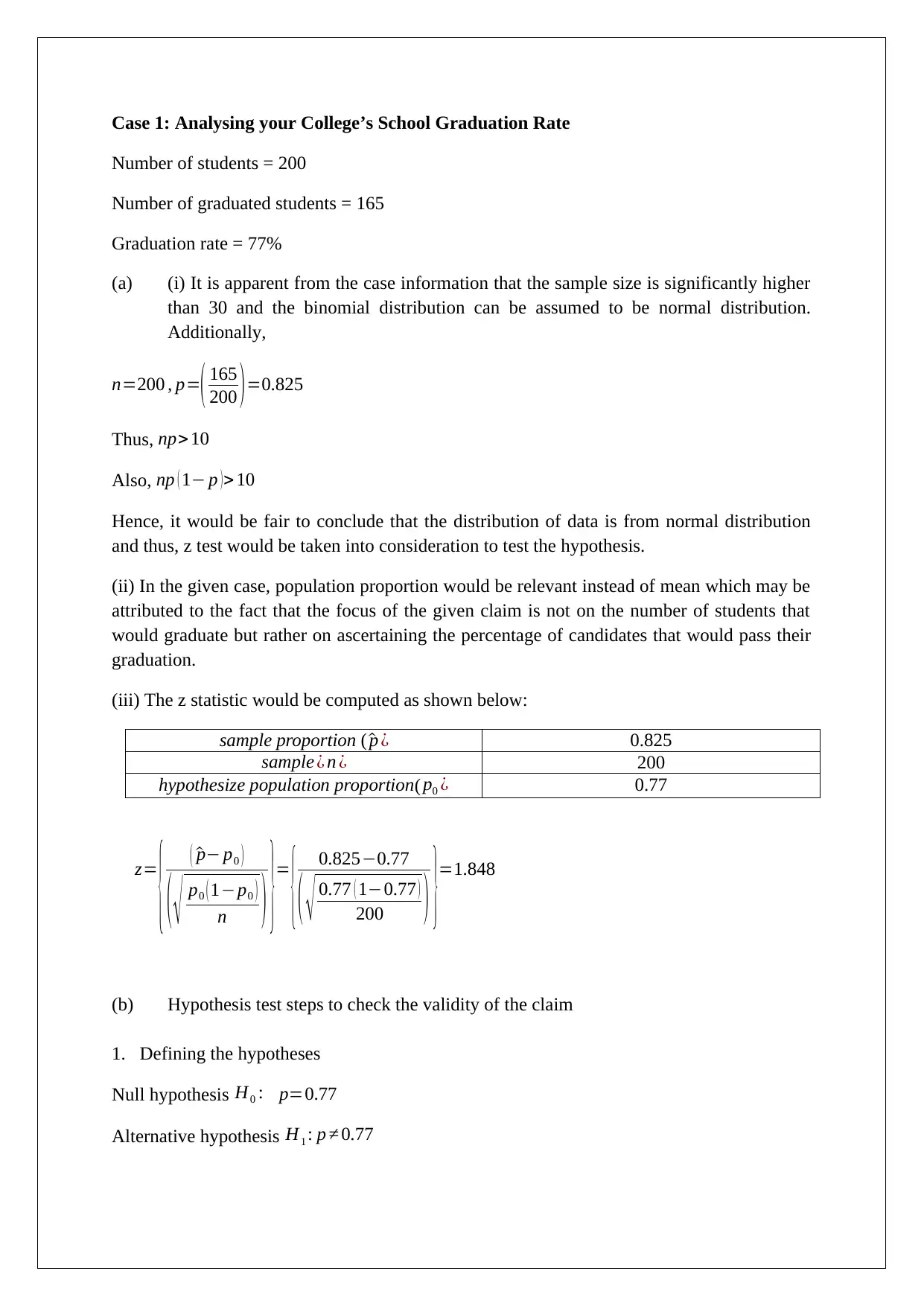
Case Study
AI Summary
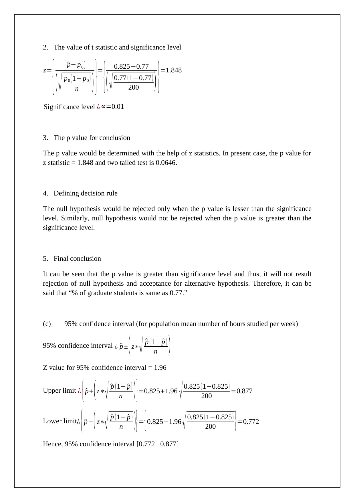
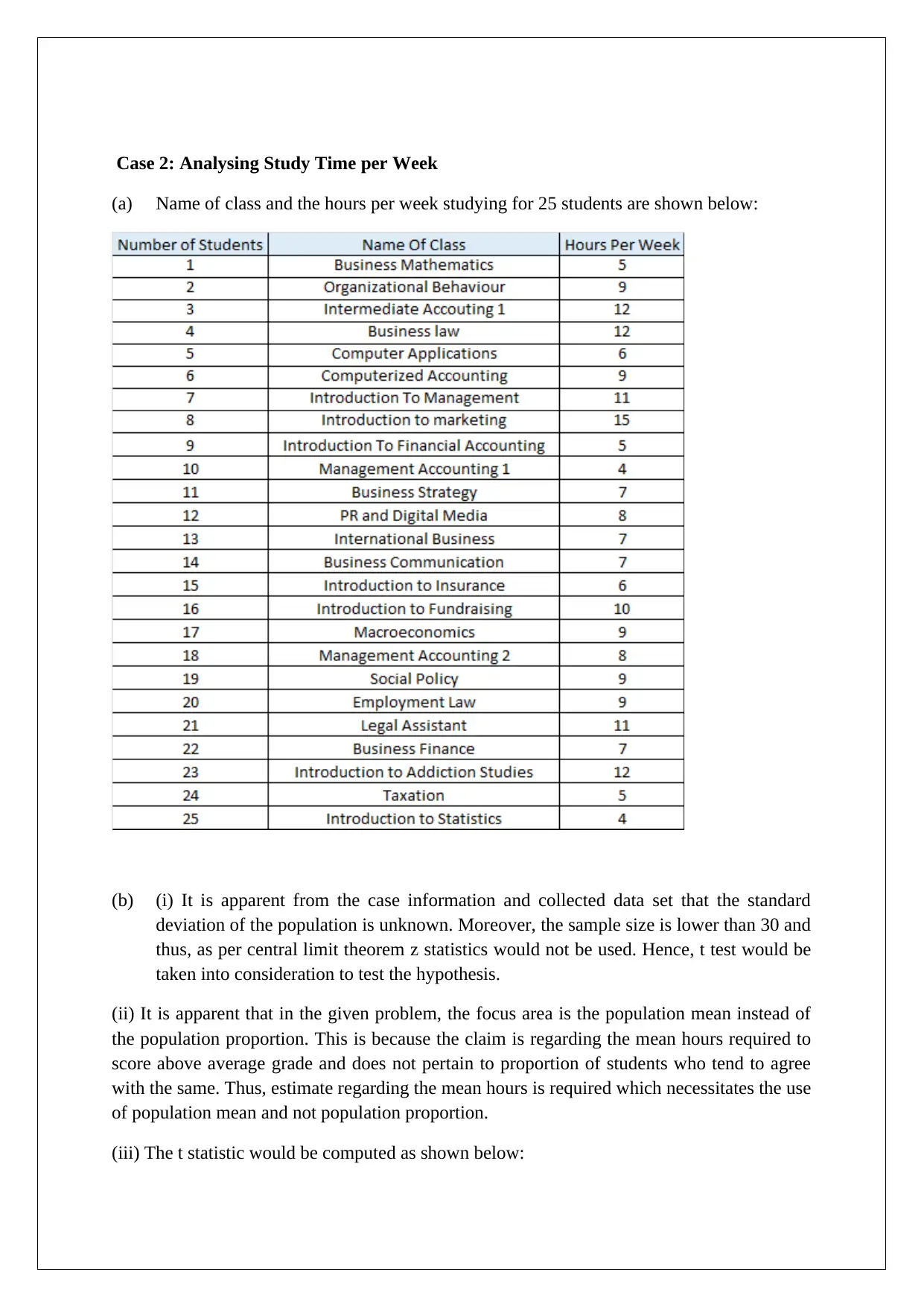
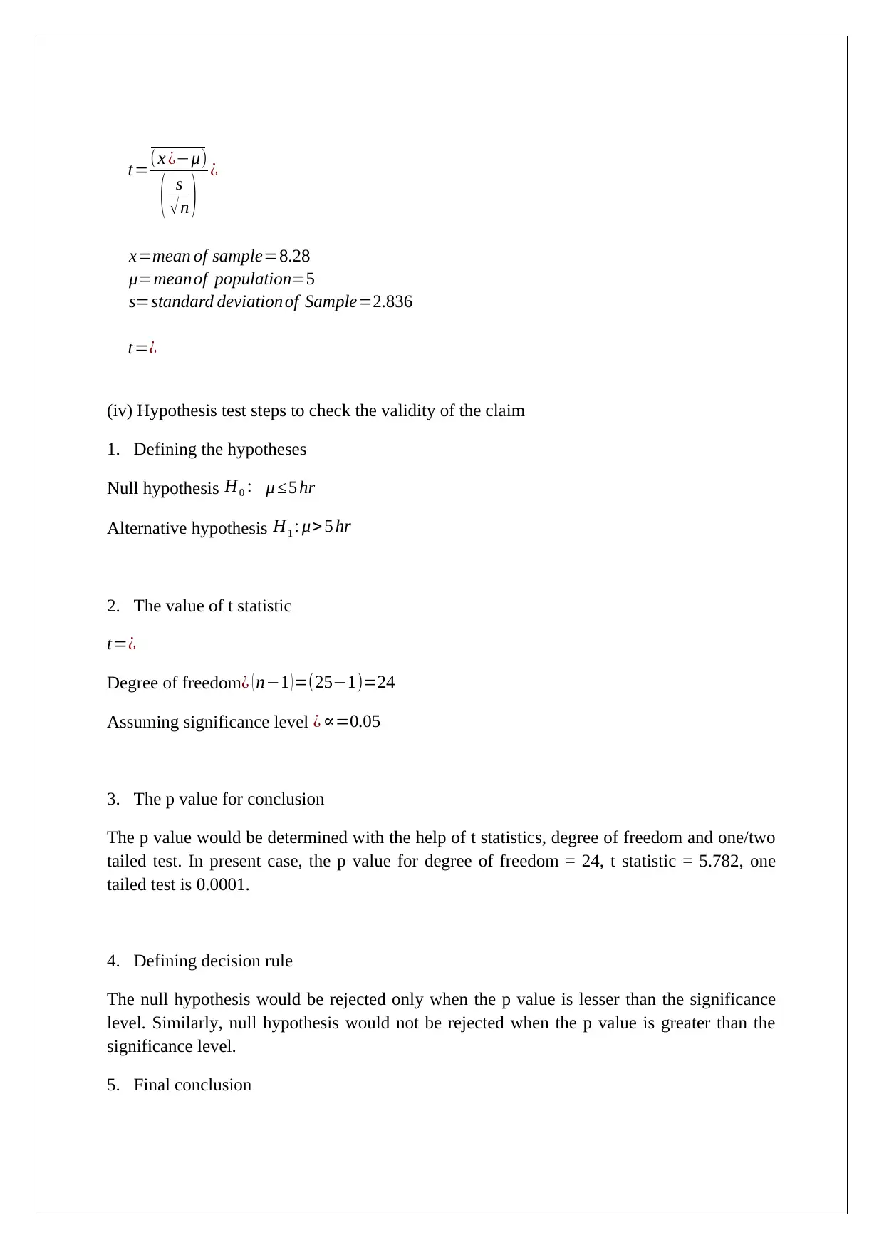
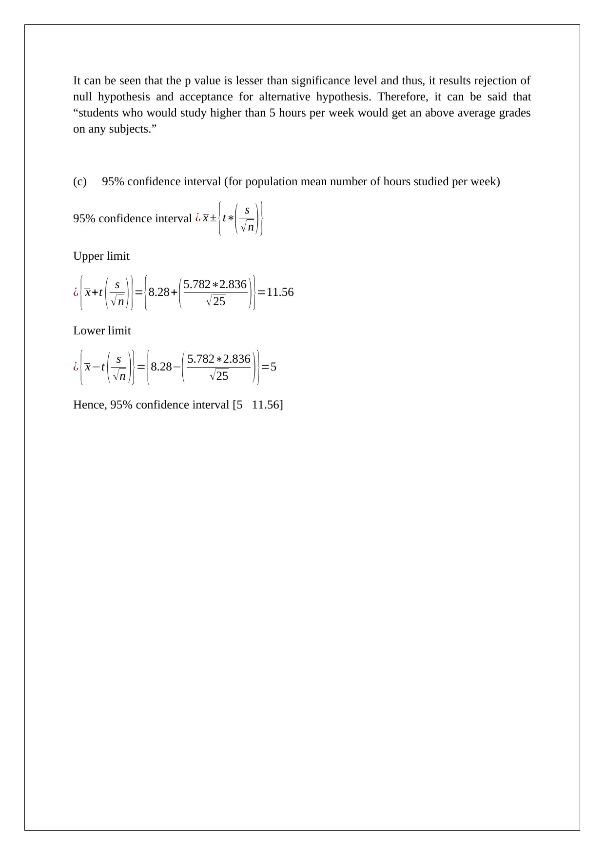
This case study analyzes two scenarios using statistical methods. Case 1 examines a college's graduation rate, employing a z-test to test a hypothesis about the proportion of graduating students. The analysis includes defining hypotheses, calculating the z-statistic, determining the p-value, establishing a decision rule, and drawing conclusions based on a 95% confidence interval. Case 2 investigates study time per week, using a t-test to evaluate the relationship between study hours and achieving above-average grades. This analysis involves defining hypotheses, calculating the t-statistic, determining the p-value, establishing a decision rule, and drawing conclusions based on a 95% confidence interval. Both cases provide a comprehensive application of statistical techniques to real-world scenarios, offering insights into data analysis and hypothesis testing.
1 out of 6
Related Documents


Your All-in-One AI-Powered Toolkit for Academic Success.
+13062052269
info@desklib.com
Available 24*7 on WhatsApp / Email
![[object Object]](/_next/static/media/star-bottom.7253800d.svg)
Copyright © 2020–2026 A2Z Services. All Rights Reserved. Developed and managed by ZUCOL.