Statistical Analysis of Wage Rates: Homework Assignment Solution

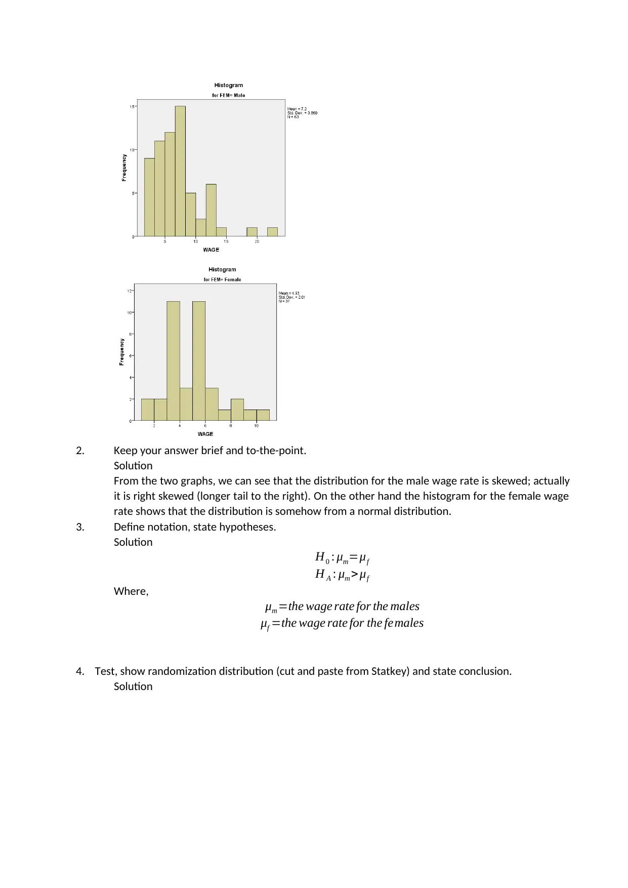
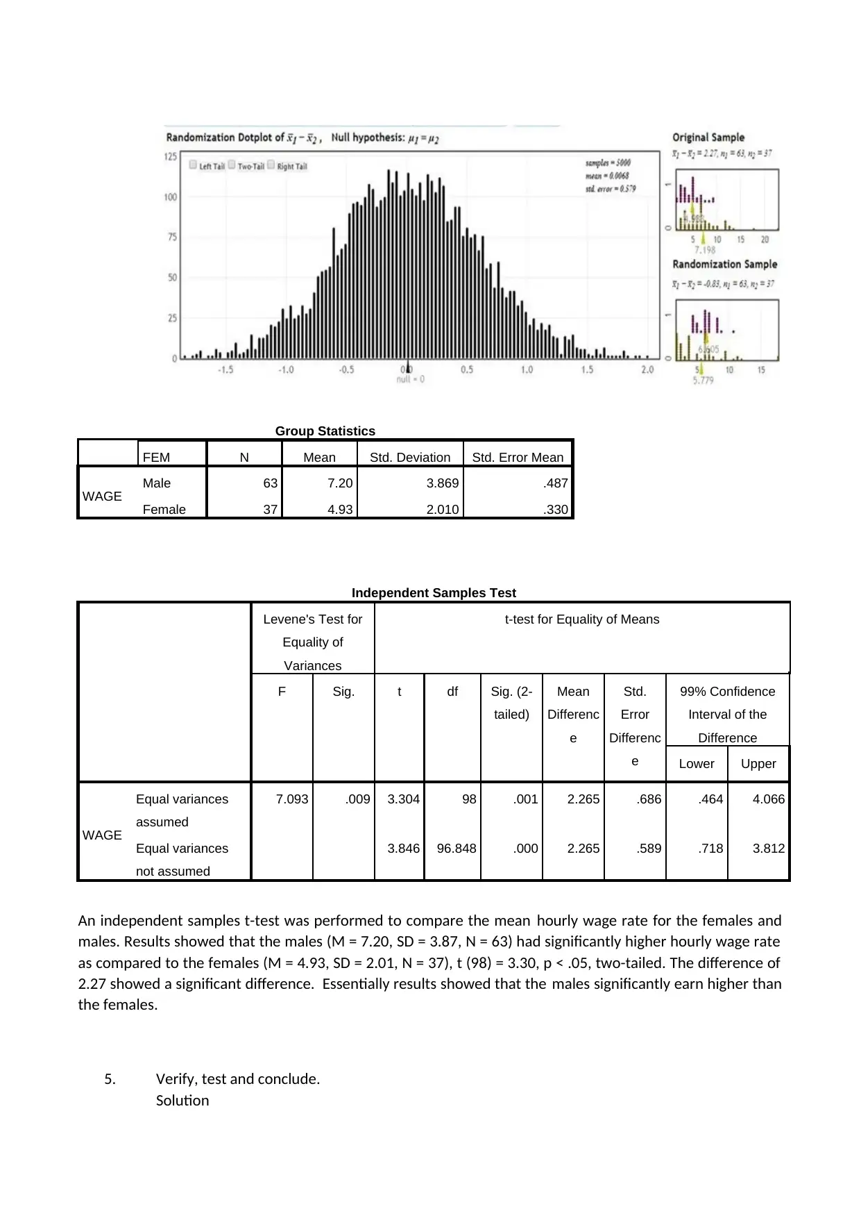
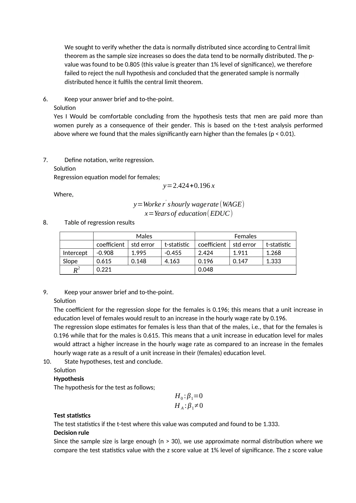
This statistics homework assignment analyzes male and female wage rates using various statistical methods. The solution begins with an observation of the wage rate distribution for both genders, identifying right-skewed distribution for males and a near-normal distribution for females. It then defines notation and states hypotheses, followed by an independent samples t-test to compare the mean hourly wage rates, which revealed that males had significantly higher wage rates. The solution also addresses the Central Limit Theorem, concluding that the sample is normally distributed. Furthermore, the assignment includes the development and interpretation of regression equations for both males and females, analyzing the impact of education level on wage rates and testing the significance of the regression slope. The analysis demonstrates the application of statistical tests and models to draw meaningful conclusions from the data.

Statistics
Name:
Institution:
7th June 2018

1. Male and female wage histograms.
Solution

2. Keep your answer brief and to-the-point.
Solution
From the two graphs, we can see that the distribution for the male wage rate is skewed; actually
it is right skewed (longer tail to the right). On the other hand the histogram for the female wage
rate shows that the distribution is somehow from a normal distribution.
3. Define notation, state hypotheses.
Solution
H0 : μm=μf
H A : μm >μf
Where,
μm =the wage rate for the males
μf =the wage rate for the females
4. Test, show randomization distribution (cut and paste from Statkey) and state conclusion.
Solution

Group Statistics
FEM N Mean Std. Deviation Std. Error Mean
WAGE Male 63 7.20 3.869 .487
Female 37 4.93 2.010 .330
Independent Samples Test
Levene's Test for
Equality of
Variances
t-test for Equality of Means
F Sig. t df Sig. (2-
tailed)
Mean
Differenc
e
Std.
Error
Differenc
e
99% Confidence
Interval of the
Difference
Lower Upper
WAGE
Equal variances
assumed
7.093 .009 3.304 98 .001 2.265 .686 .464 4.066
Equal variances
not assumed
3.846 96.848 .000 2.265 .589 .718 3.812
An independent samples t-test was performed to compare the mean hourly wage rate for the females and
males. Results showed that the males (M = 7.20, SD = 3.87, N = 63) had significantly higher hourly wage rate
as compared to the females (M = 4.93, SD = 2.01, N = 37), t (98) = 3.30, p < .05, two-tailed. The difference of
2.27 showed a significant difference. Essentially results showed that the males significantly earn higher than
the females.
5. Verify, test and conclude.
Solution

We sought to verify whether the data is normally distributed since according to Central limit
theorem as the sample size increases so does the data tend to be normally distributed. The p-
value was found to be 0.805 (this value is greater than 1% level of significance), we therefore
failed to reject the null hypothesis and concluded that the generated sample is normally
distributed hence it fulfils the central limit theorem.
6. Keep your answer brief and to-the-point.
Solution
Yes I Would be comfortable concluding from the hypothesis tests that men are paid more than
women purely as a consequence of their gender. This is based on the t-test analysis performed
above where we found that the males significantly earn higher than the females (p < 0.01).
7. Define notation, write regression.
Solution
Regression equation model for females;
y=2.424+0.196 x
Where,
y=Worke r' s hourly wagerate (WAGE)
x=Years of education( EDUC )
8. Table of regression results
Males Females
coefficient std error t-statistic coefficient std error t-statistic
Intercept -0.908 1.995 -0.455 2.424 1.911 1.268
Slope 0.615 0.148 4.163 0.196 0.147 1.333
R2 0.221 0.048
9. Keep your answer brief and to-the-point.
Solution
The coefficient for the regression slope for the females is 0.196; this means that a unit increase in
education level of females would result to an increase in the hourly wage rate by 0.196.
The regression slope estimates for females is less than that of the males, i.e., that for the females is
0.196 while that for the males is 0.615. This means that a unit increase in education level for males
would attract a higher increase in the hourly wage rate as compared to an increase in the females
hourly wage rate as a result of a unit increase in their (females) education level.
10. State hypotheses, test and conclude.
Solution
Hypothesis
The hypothesis for the test as follows;
H0 : β1=0
H A : β1 ≠ 0
Test statistics
The test statistics if the t-test where this value was computed and found to be 1.333.
Decision rule
Since the sample size is large enough (n > 30), we use approximate normal distribution where we
compare the test statistics value with the z score value at 1% level of significance. The z score value

at 1% level of significance is 2.58. The computed test statistics (t-value) is 1.333. Since the computed
value is less than the z critical value, we fail to reject the null hypothesis.
Conclusion
By failing to reject the null hypothesis we conclude that the regression slope is not different from
zero and as such we conclude that education is not an effective predictor of female wage rates in the
regression model