[PDF] Univariate and Multivariate Analysis of Variance
VerifiedAdded on 2020/10/22
|30
|5077
|453
AI Summary
The provided assignment involves analyzing the variance of a dependent variable 'year' using univariate and multivariate statistical methods. A univariate analysis is conducted on the variable 'year', including profile plots and tests of between-subjects effects. The study also explores the factors affecting 'year' in relation to independent variables 'BCratio' and 'Ontarioratio'.
Contribute Materials
Your contribution can guide someone’s learning journey. Share your
documents today.

PROJECT
Secure Best Marks with AI Grader
Need help grading? Try our AI Grader for instant feedback on your assignments.
TABLE OF CONTENTS
INTRODUCTION...........................................................................................................................1
OBJECTIVE....................................................................................................................................1
LITERATURE REVIEW................................................................................................................1
METHODOLOGY AND DESCRIPTION OF DATA...................................................................3
EMPIRICAL RESULTS..................................................................................................................4
DISCUSSION..................................................................................................................................4
CONCLUSION AND RECOMMENDATION ..............................................................................5
FUTURE RESEARCH....................................................................................................................6
REFERENCES................................................................................................................................7
APPENDIX......................................................................................................................................8
INTRODUCTION
Title: A study on Average and median gender wage ratio in Canada”
Income inequality is replicated as extreme concentration of income or wealth with small
percentage of population. It is the extent where income is distributed unevenly in particular
country as this is very significant indicator of equity in economy and has presence of
implications for other social results like crime and life satisfaction. It has been articulated as
contributing factor to gender wage gap for multiple decades. In Canada, there in increment in
average income he bottom 90% of income group prior to adjusting for inflation. Conversely,
average income among top 1% has rose over similar duration and this disproportionate raises in
top income have multiple consequences for overall gender wage gap due to representation of
women in top income groups (Anderson and et.al., 2019). This paper will give brief study on
average and median gender wage ratio in Canada with context to Quebec, Ontario and British
Columbia.
The Gender wage gap is considered as difference in earnings of men and women at
workplace. This is broadly recognised as indicator of economic equality of women along with
existence to some extent in every country throughout the world. The data would be gathered
from 1990 to 2011 for attaining the objective of research.
OBJECTIVE
This research is performed for evaluating average and median gender wage ratio in
Canada. It is on basis of assumption that gender wage ratio would be influenced through income
inequality.
Hypothesis
H0: Null hypothesis: There is no statistical significant difference in the mean value of female to
male earnings ratio with regards to Quebec, Ontario and British Columbia.
H1: Alternative hypothesis: There is a statistical significant difference in the mean value of
female to male earnings ratio with regards to Quebec, Ontario and British Columbia.
LITERATURE REVIEW
According to Card, Lemieux and Riddell (2018), since year 1981, gender pay gap is
difference among earnings of male and female which is expressed as proportion of earnings of
male. It has decreased by 21% in Canada with various decrease occurring prior to year 2011.
There are numerous trends which had occurred in post World War II which had contributed for
1
purpose of improvements in gender pay gap. Further, labour force participation of women has
raised on significant basis and driven simultaneously through raise in proportion of employed
women and fall in propensity of employed women for withdrawing workforce on motherhood or
marriage. However, Beaudoin (2018) had argued that women have entered workforce with
higher education with formation of substantial gain in attainment of education over past decades
with increasingly acquired post secondary education, specifically at university's degree at
bachelor or above the level. At the current state, females have also decreased the time of their
interruptions related to family work like child care, pregnancy, partner's job and relocating for
their spouse so that they might have more work experience compared to case in the past. In the
same series, social policy support for purpose of employment of women in terms of job protected
maternity along with parental leave along with replacement of partial income for expansion of
leave with legislation addressing labour market's unfair treatment.
As per views of Javdani and McGee (2019), pay inequality among male and female is a
persistent phenomenon as per labour force survey, 70.2% female aged 15 years and older in
Canada had participated and this which shows that $0.87 for each dollar earned through men
measured with similar number of hours. The Equal pay day is used in different countries for
spreading awareness related to gender pay gap. On basis of gender pay gap of country, equal pay
day is considered as date which symbolise that when women must be stop for getting paid for
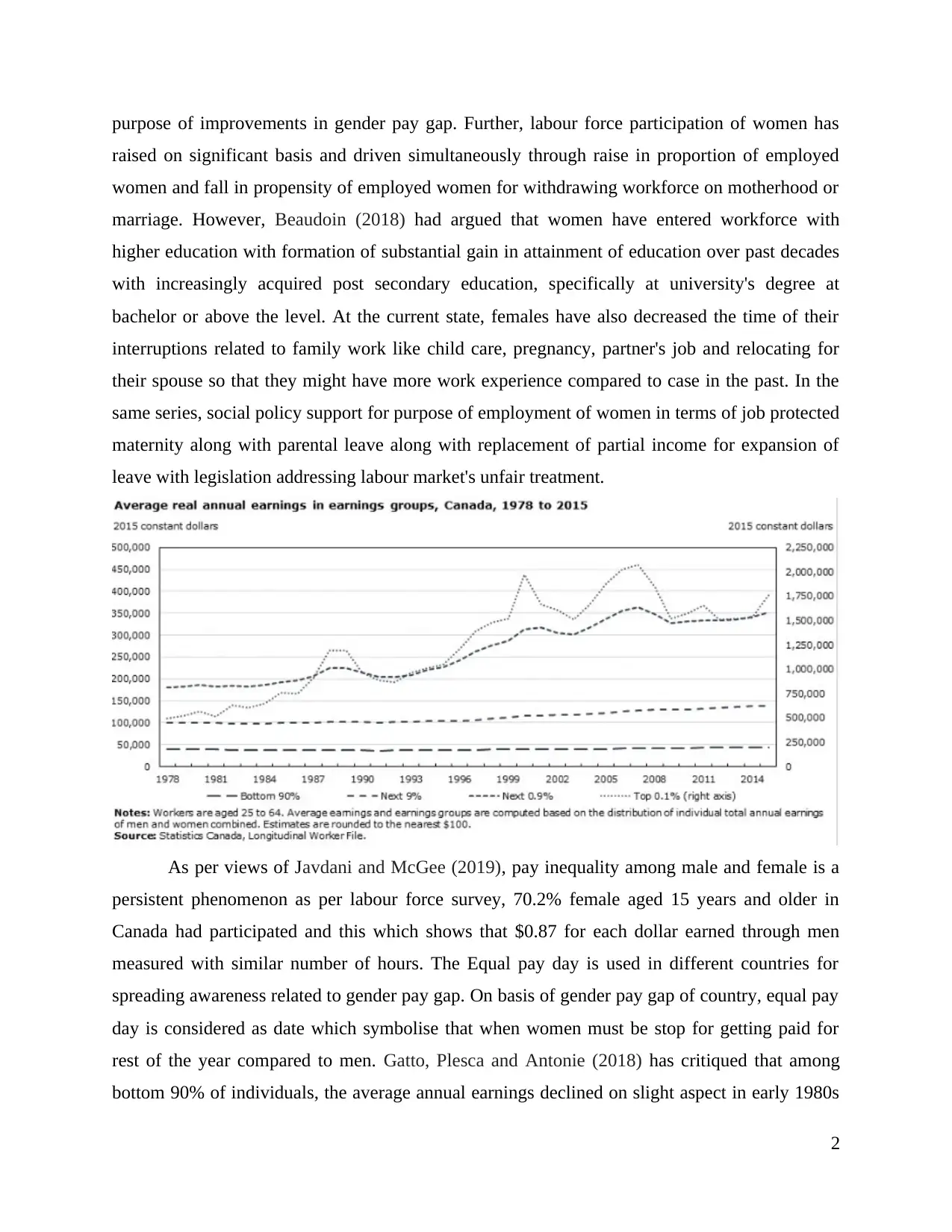
rest of the year compared to men. Gatto, Plesca and Antonie (2018) has critiqued that among
bottom 90% of individuals, the average annual earnings declined on slight aspect in early 1980s
2
Secure Best Marks with AI Grader
Need help grading? Try our AI Grader for instant feedback on your assignments.
and remained at $37000 through much of the rest of 1980s and early 1990 which has gradual
raise around $44000 by the mid stage of 2010. From the period of 1978 to year 2011, the average
annual earnings within group has raised with average of 0.3% each year.
Among the next 9%, this had decreased slightly around $98000 in early 1980s and
increased with $137000 by mid of 2010s and gain over year with averaging 0.9% over the
period. Further, next 0.9% the average annual gains were twice of past group at 1.9% every year
with average earning from $180000 in early mid 1980s to over $350000 in year 2015. As per
views of Hara (2018), in terms of timing, next 9% had faced smaller growth in the 1980s
compared to 19910 by 0.2% and 0.9% respectively. The average earnings of the next 0.9% and
very important of top 0.1% had reached peak around year 2000 at dot-com bubble and before
global crisis in year 2007. Till early 2010s, earnings of top groups had returned to level observed
in mid 2000s.
According to views of Behr and Theune (2018), the impact of trends on overall gender
earnings gap is identified through two factors such as earnings of women relative to those of men
within every group and representation of women within every earnings group. Both of these
factors are appropriately addressed in analysis. The share of female in group of top earnings
raised with consideration of over the period from 1978 to 2015. On the contrary, Buchanan,
McFarlane and Das (2018) stated that female are significantly under represented in every group
by end of period. From the mid of 2000s onwards, female accounted for 48% of every earners
and just over 50% or earners in bottom 90%. Simultaneously, it has been clearly stated that gains
made in women representation and apart from this women left significantly under represented in
every top earnings group. The annual earnings of women relative to those of men which varied
across the top earnings of group. The women's and men's earnings are compared and bounded
through top and bottom with similar thresholds.
Consequently, if male and female were equally likely to attain these earnings groups,
with range of possibilities of annual earnings in every group is large that one will not expect
average earnings of female and male to be automatically equalized and disappearance of pay
gap.
METHODOLOGY AND DESCRIPTION OF DATA
The analysis has been performed with application of three way anova as this is used for
identifying that there is presence of interaction effect among three independent variables on a
3
continuous dependent variable. This is extension of two way anova which just reflects interaction
in two independent variables. It is also known as three factor Anova as it is statical mode to
identify their effect on three factors of the outcome With use of this method, there is retained of
adjusted p values along with critical F values per family error rate. Moreover, there is used of
SPSS syntax to obtain outcome of three way anova.
With reference to our artificial data set replicated as three way has presence of statistical
significant three way interaction for purpose of illustrating the process. In our data set, variables
Quebec, Ontario and British Columbia are categorical variable. For purpose of performing this
interaction, firstly there is extraction of two way interaction to perform in depth analysis. There
would be examination of year to Quebecratio * Ontarioratio interaction, Quebecratio * British
Columbia interaction and British Columbia * Ontarioratio interaction.
Apart from this, there is presence of numerous assumptions as its dependent variable
which must be measures at continuous level which is year in particular data set. On basis of
independent variables Quebec, Ontario and British Columbia are categorical variable with
absence of significant outliers.
EMPIRICAL RESULTS
While analysing, its results it has been extracted that Quebecratio and Ontarioratio is
about 0.126 which shows that it is greater than 0.05 (0.126 > 0.05) so null hypothesis is accepted.
In simple words, it could be elaborated that there is no statistical significant difference in the
mean value of female to male earnings ratio with regards to Quebec and Ontario. When there is
presence of statistical significant interaction had reported main effected could be misleading. So,
with this context, there is requirement of engaging to identify mean difference in Qubec, Ontario
and British Columbia.
DISCUSSION
On basis of above study, it had been discussed that Canadian women had earned 87% and
gender parity has attained in public sector. The Canadian women are less likely for being
employed compared to Canadian men. In simpler terms, gender pay gap is variation among
wages earned through men and women. The recent statistics of Canada reflects that gender wage
Gap in Ontario is 26% and in simpler terms this could be elaborated that each male earned $1
and on similar note female earned 74 cents. In year 1987, when pay Equity Act was passed then
gender wage gap was about 36%. It has been narrowed on slower aspect over the time and Pay
4
equity Office has continued its ongoing efforts for correcting and monitoring gender wage gap
for women workers of Ontario.
It has articulated trends incur in Post World war II which contributes for major
modifications in gender pay gap. The female workers have started working with high education
and develops substantial gain to accomplish education over past decades along with getting post
secondary education. In the present scenario, women have reduced time of their family related
work interruptions such as pregnancy, relocation due to partner's job, child care and many more.
Further, there is observance of social policy support regarding employment of women in form of
job protected maternity and parental leave for replacement of partial income for leave expansion
which addresses unfair treatment of labour market. In simpler words, it is very significant for
purpose of acknowledging potential pitfalls linked with different counterfactuals. The main
emphasis is on under-representation of women in top decile on overall average gender pay gap. It
has been observed that average and median earning of both gender male and female within every
group changes.
Furthermore, under-representation of women in top earners had appeared for accounting
growth portion of the gap of gender earnings. From year 1978 to 1980, under representation of
female in top earners had accounted approx 41% of gender earnings gap and from 2001 to 2015,
it is all about 60% at an average.
CONCLUSION AND RECOMMENDATION
From the above report it had been concluded that income inequality plays major role in
gender pay wage ratio in every country. Moreover, it has shown that women with similar
experience, demographic and socio economic background earn approx $7200 less than men
counterparts per year. Aggregating this annually this amount gives significant impact on
women's economic stability and reduce financial interdependence along with capability for
saving for their retirement. In the same series, it has shown that gender wage gap is very
complex and outcomes through multiple factors like tradition “women's work” pays less
compared to traditional “men's work” and second is about most women workers are directly
employed in occupation which are lower wage and industries which pays lower.
It has been recommended to close gender wage gap in Canada as to encourage female to
seek employment in occupations of higher wage. The females must be encourage for pursuing
higher degree in traditionally fields where male are dominated like science, engineering,
5
Paraphrase This Document
Need a fresh take? Get an instant paraphrase of this document with our AI Paraphraser
mathematics and engineering can create unique image. Early exposure of young female to these
subjects helps in field and for mentorship programs. Apart from this, good management
contributes big role to attract and retain highly skilled female as its application is to every field
such as engineering, high skilled and higher wage occupations.
Simultaneously, improvement in policies of workplace can also make difference such as
flexible hours, parental leave and telecommuting helps female balance demand of family and
work as well. Organizations could address problems only if there is existence and this could be
attained through tracing and disclosing information on promotions, recruitment and promotions.
FUTURE RESEARCH
This research is very useful for purpose of further researchers to evaluate the past data
and current trends. Simultaneously, after this there could be application of research on
government policies which are supporting income inequality and gender pay wage gap ratio.
Apart from this, research on basis of organizations which are undertaking actions for high skilled
job for women and avoiding discrimination among male and female along with parental leave.
6
REFERENCES
Books and Journals
Anderson, D. and et.al., 2019. On a Firm’s Optimal Response to Pressure for Gender Pay
Equity. Organization Science.
Beaudoin, J. D., 2018. Minding the Gap: Pay Equity and the Role of Law in Narrowing
Canada's Gender Wage Gap(Doctoral dissertation, The University of Western Ontario).
Behr, A. and Theune, K., 2018. The gender pay gap at labour market entrance: Evidence from
Germany. International Labour Review. 157(1). pp.83-100.
Buchanan, T., McFarlane, A. and Das, A., 2018. Educational Attainment and the Gender Gap in
Childcare in Canada: A Decomposition Analysis. Margin: The Journal of Applied
Economic Research. 12(4). pp.458-476.
Card, D., Lemieux, T. and Riddell, W. C., 2018. Unions and Wage Inequality: The Roles of
Gender, Skill and Public Sector Employment (No. w25313). National Bureau of Economic
Research.
Gatto, L., Plesca, M. and Antonie, L., 2018, September. Gender Wage Gap in the University
Sector: A Case Study of All Universities in Ontario, Canada. In International Conference
on Social Informatics (pp. 242-256). Springer, Cham.
Hara, H., 2018. The gender wage gap across the wage distribution in Japan: Within-and
between-establishment effects. Labour Economics. 53. pp.213-229.
Javdani, M. and McGee, A., 2019. Moving Up or Falling Behind? Gender, Promotions, and
Wages in Canada. Industrial Relations: A Journal of Economy and Society.
7
APPENDIX
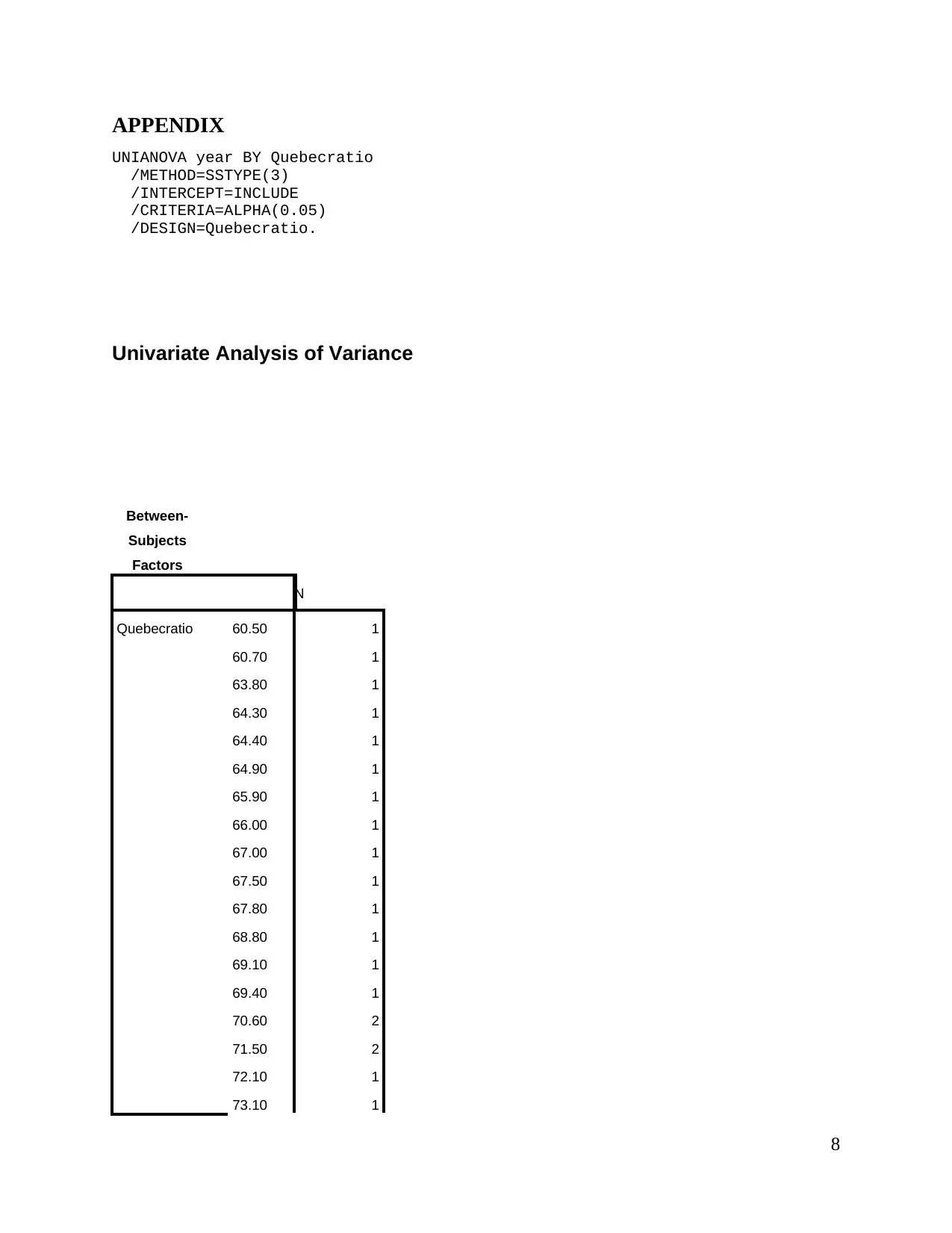
UNIANOVA year BY Quebecratio
/METHOD=SSTYPE(3)
/INTERCEPT=INCLUDE
/CRITERIA=ALPHA(0.05)
/DESIGN=Quebecratio.
Univariate Analysis of Variance
Between-
Subjects
Factors
N
Quebecratio 60.50 1
60.70 1
63.80 1
64.30 1
64.40 1
64.90 1
65.90 1
66.00 1
67.00 1
67.50 1
67.80 1
68.80 1
69.10 1
69.40 1
70.60 2
71.50 2
72.10 1
73.10 1
8
Secure Best Marks with AI Grader
Need help grading? Try our AI Grader for instant feedback on your assignments.
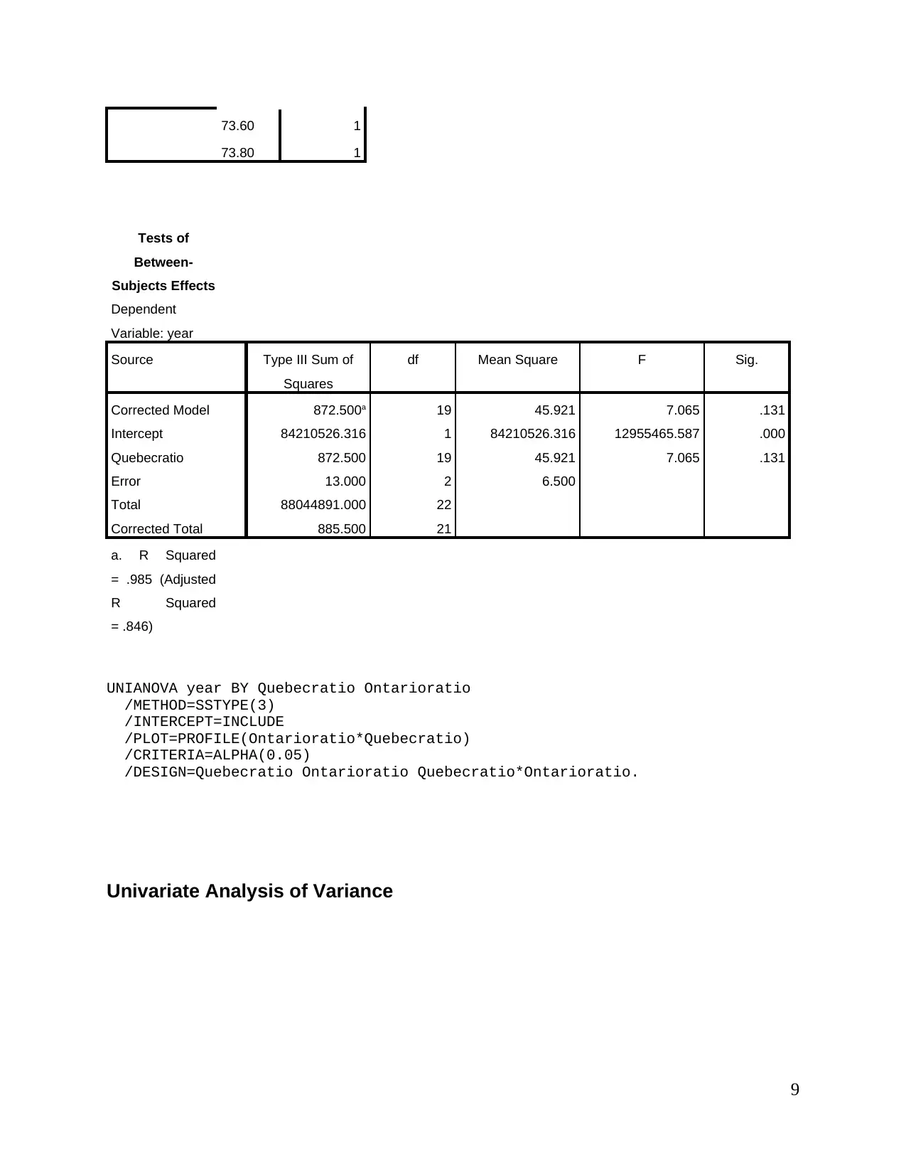
73.60 1
73.80 1
Tests of
Between-
Subjects Effects
Dependent
Variable: year
Source Type III Sum of
Squares
df Mean Square F Sig.
Corrected Model 872.500a 19 45.921 7.065 .131
Intercept 84210526.316 1 84210526.316 12955465.587 .000
Quebecratio 872.500 19 45.921 7.065 .131
Error 13.000 2 6.500
Total 88044891.000 22
Corrected Total 885.500 21
a. R Squared
= .985 (Adjusted
R Squared
= .846)
UNIANOVA year BY Quebecratio Ontarioratio
/METHOD=SSTYPE(3)
/INTERCEPT=INCLUDE
/PLOT=PROFILE(Ontarioratio*Quebecratio)
/CRITERIA=ALPHA(0.05)
/DESIGN=Quebecratio Ontarioratio Quebecratio*Ontarioratio.
Univariate Analysis of Variance
9
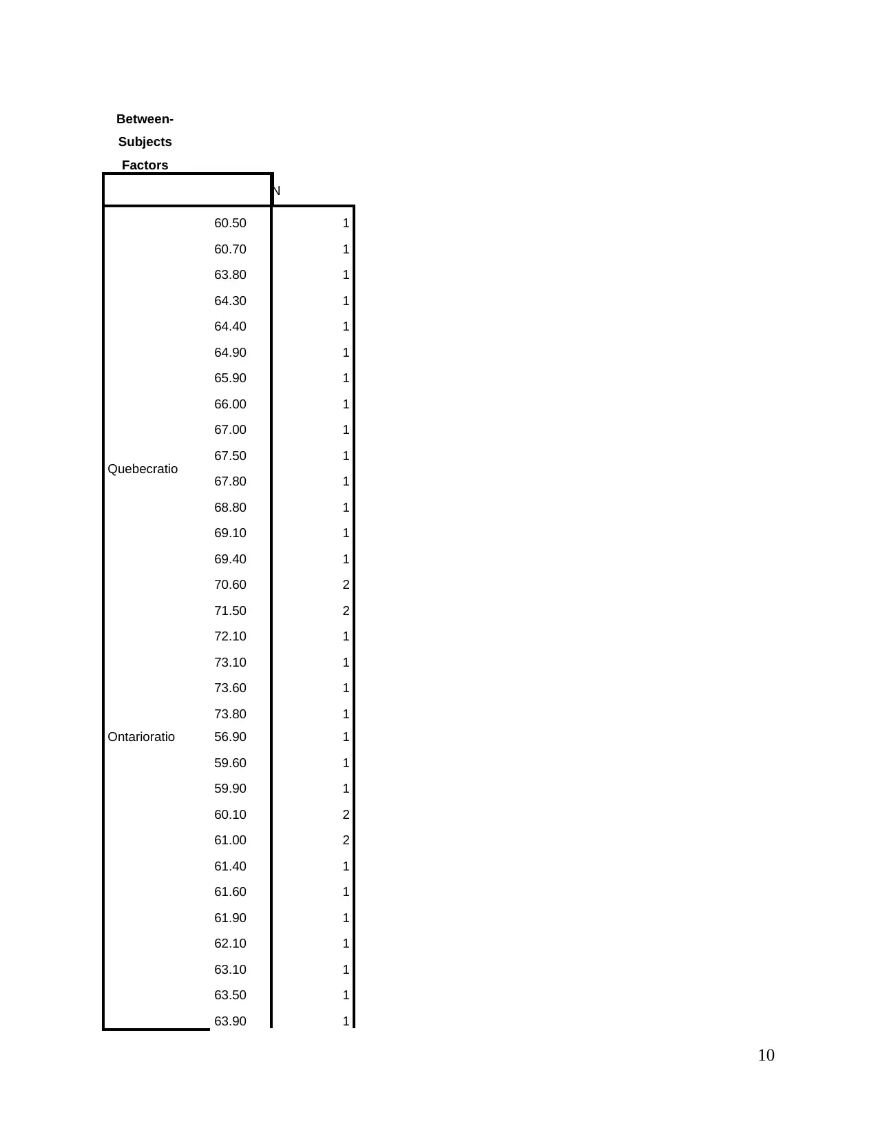
Between-
Subjects
Factors
N
Quebecratio
60.50 1
60.70 1
63.80 1
64.30 1
64.40 1
64.90 1
65.90 1
66.00 1
67.00 1
67.50 1
67.80 1
68.80 1
69.10 1
69.40 1
70.60 2
71.50 2
72.10 1
73.10 1
73.60 1
73.80 1
Ontarioratio 56.90 1
59.60 1
59.90 1
60.10 2
61.00 2
61.40 1
61.60 1
61.90 1
62.10 1
63.10 1
63.50 1
63.90 1
10
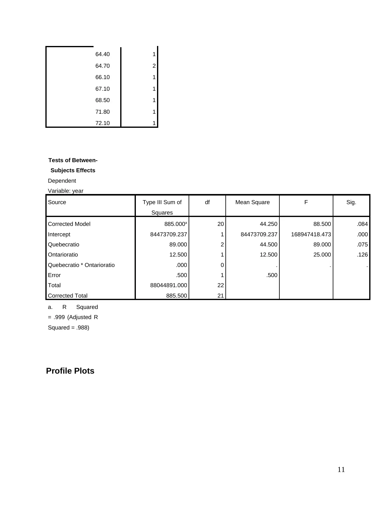
64.40 1
64.70 2
66.10 1
67.10 1
68.50 1
71.80 1
72.10 1
Tests of Between-
Subjects Effects
Dependent
Variable: year
Source Type III Sum of
Squares
df Mean Square F Sig.
Corrected Model 885.000a 20 44.250 88.500 .084
Intercept 84473709.237 1 84473709.237 168947418.473 .000
Quebecratio 89.000 2 44.500 89.000 .075
Ontarioratio 12.500 1 12.500 25.000 .126
Quebecratio * Ontarioratio .000 0 . . .
Error .500 1 .500
Total 88044891.000 22
Corrected Total 885.500 21
a. R Squared
= .999 (Adjusted R
Squared = .988)
Profile Plots
11
Paraphrase This Document
Need a fresh take? Get an instant paraphrase of this document with our AI Paraphraser
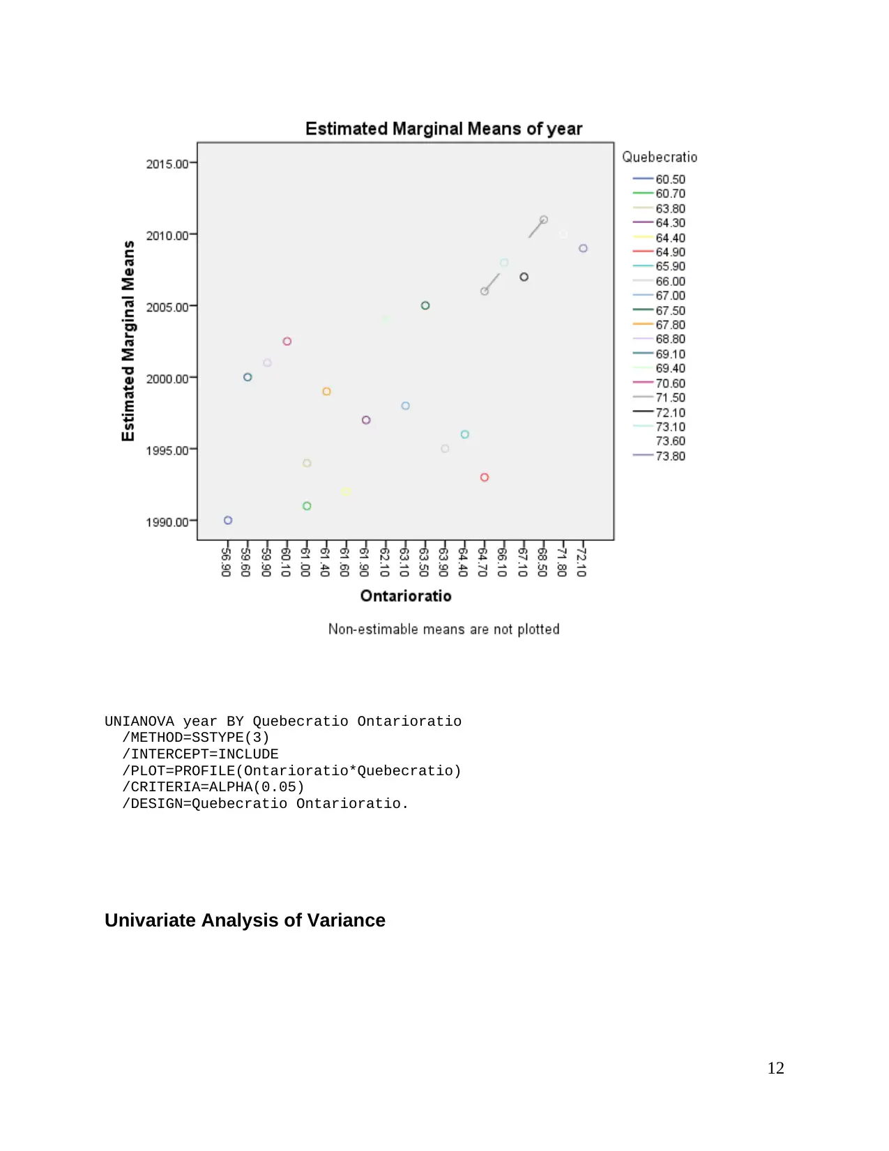
UNIANOVA year BY Quebecratio Ontarioratio
/METHOD=SSTYPE(3)
/INTERCEPT=INCLUDE
/PLOT=PROFILE(Ontarioratio*Quebecratio)
/CRITERIA=ALPHA(0.05)
/DESIGN=Quebecratio Ontarioratio.
Univariate Analysis of Variance
12
/METHOD=SSTYPE(3)
/INTERCEPT=INCLUDE
/PLOT=PROFILE(Ontarioratio*Quebecratio)
/CRITERIA=ALPHA(0.05)
/DESIGN=Quebecratio Ontarioratio.
Univariate Analysis of Variance
12
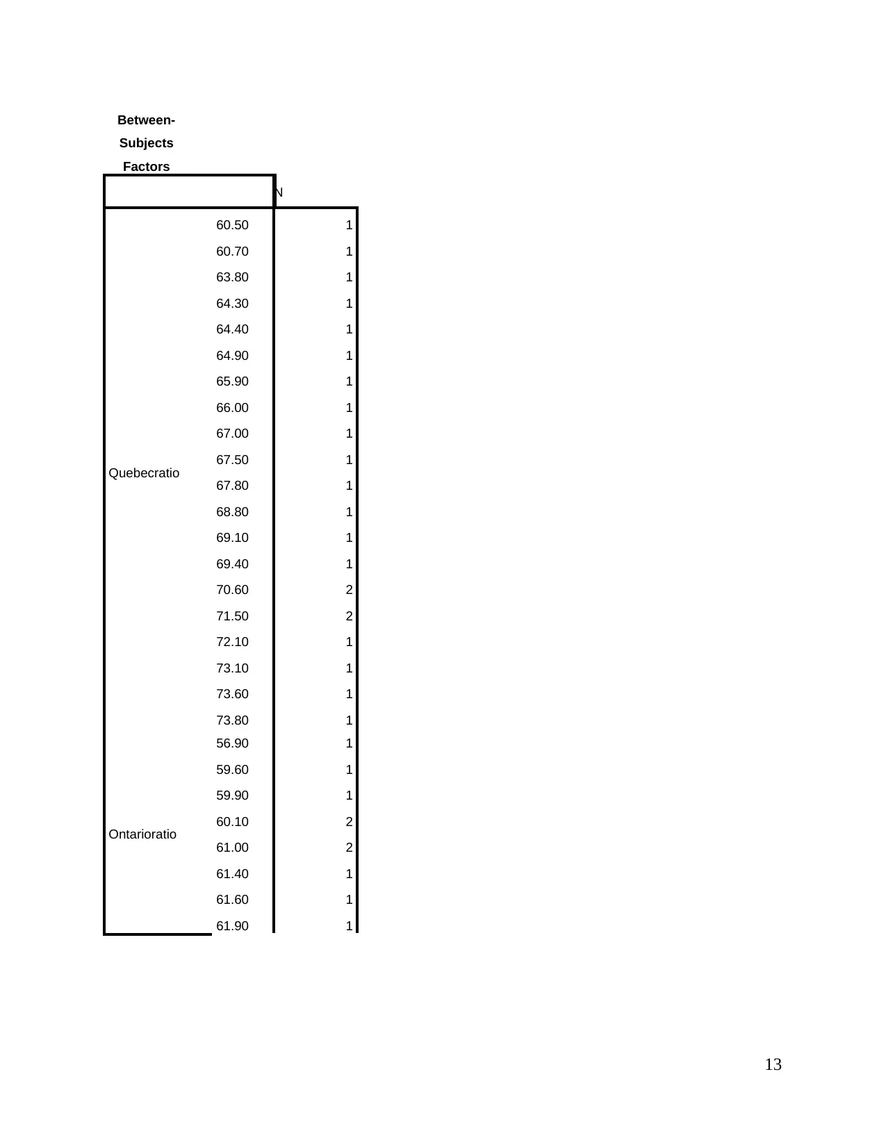
Between-
Subjects
Factors
N
Quebecratio
60.50 1
60.70 1
63.80 1
64.30 1
64.40 1
64.90 1
65.90 1
66.00 1
67.00 1
67.50 1
67.80 1
68.80 1
69.10 1
69.40 1
70.60 2
71.50 2
72.10 1
73.10 1
73.60 1
73.80 1
Ontarioratio
56.90 1
59.60 1
59.90 1
60.10 2
61.00 2
61.40 1
61.60 1
61.90 1
13
Subjects
Factors
N
Quebecratio
60.50 1
60.70 1
63.80 1
64.30 1
64.40 1
64.90 1
65.90 1
66.00 1
67.00 1
67.50 1
67.80 1
68.80 1
69.10 1
69.40 1
70.60 2
71.50 2
72.10 1
73.10 1
73.60 1
73.80 1
Ontarioratio
56.90 1
59.60 1
59.90 1
60.10 2
61.00 2
61.40 1
61.60 1
61.90 1
13
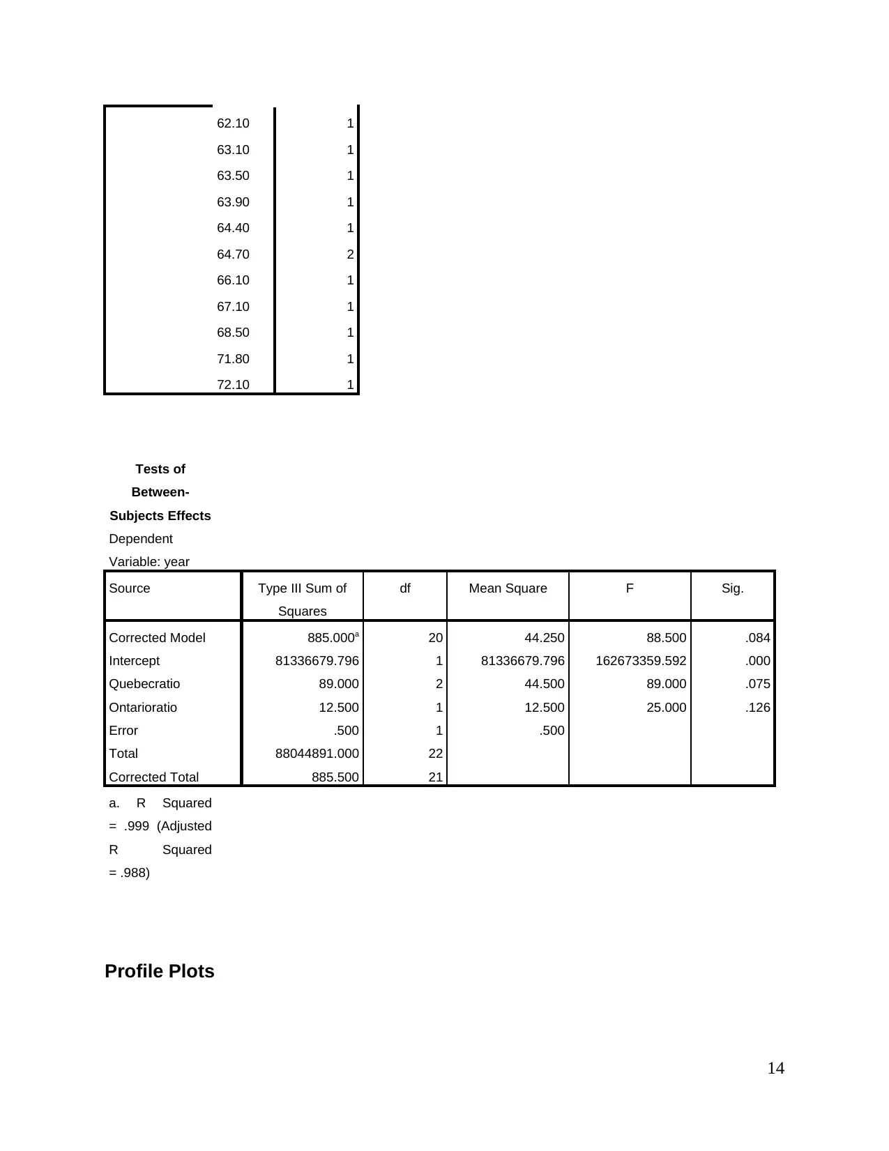
62.10 1
63.10 1
63.50 1
63.90 1
64.40 1
64.70 2
66.10 1
67.10 1
68.50 1
71.80 1
72.10 1
Tests of
Between-
Subjects Effects
Dependent
Variable: year
Source Type III Sum of
Squares
df Mean Square F Sig.
Corrected Model 885.000a 20 44.250 88.500 .084
Intercept 81336679.796 1 81336679.796 162673359.592 .000
Quebecratio 89.000 2 44.500 89.000 .075
Ontarioratio 12.500 1 12.500 25.000 .126
Error .500 1 .500
Total 88044891.000 22
Corrected Total 885.500 21
a. R Squared
= .999 (Adjusted
R Squared
= .988)
Profile Plots
14
Secure Best Marks with AI Grader
Need help grading? Try our AI Grader for instant feedback on your assignments.
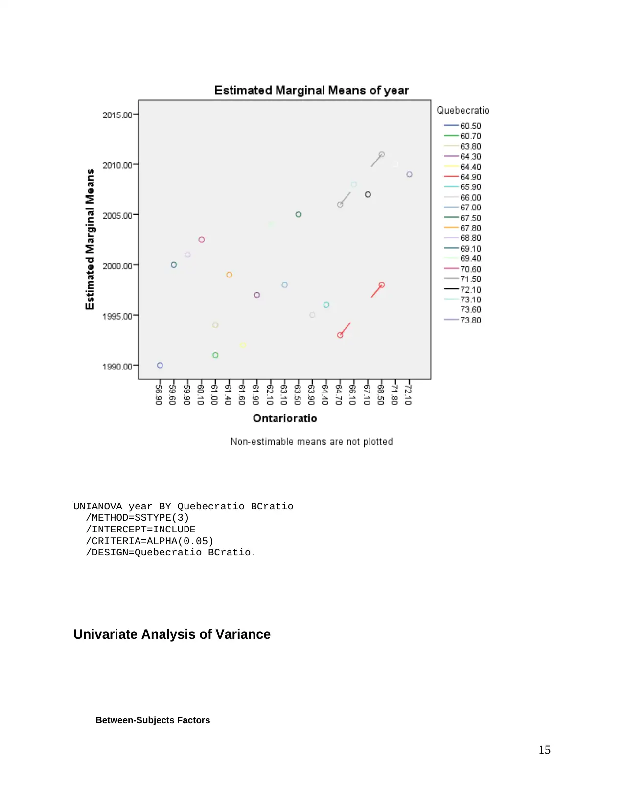
UNIANOVA year BY Quebecratio BCratio
/METHOD=SSTYPE(3)
/INTERCEPT=INCLUDE
/CRITERIA=ALPHA(0.05)
/DESIGN=Quebecratio BCratio.
Univariate Analysis of Variance
Between-Subjects Factors
15
/METHOD=SSTYPE(3)
/INTERCEPT=INCLUDE
/CRITERIA=ALPHA(0.05)
/DESIGN=Quebecratio BCratio.
Univariate Analysis of Variance
Between-Subjects Factors
15
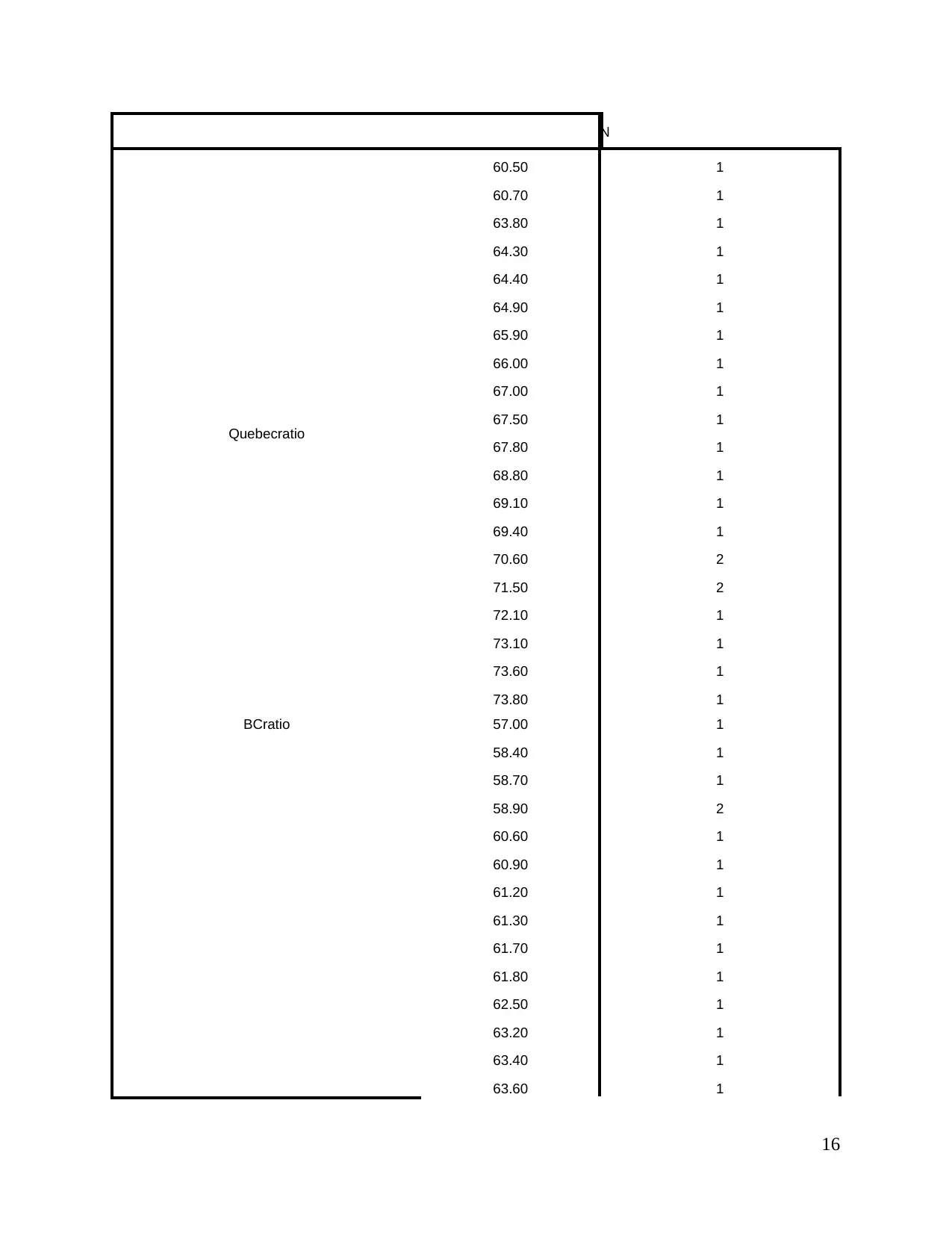
N
Quebecratio
60.50 1
60.70 1
63.80 1
64.30 1
64.40 1
64.90 1
65.90 1
66.00 1
67.00 1
67.50 1
67.80 1
68.80 1
69.10 1
69.40 1
70.60 2
71.50 2
72.10 1
73.10 1
73.60 1
73.80 1
BCratio 57.00 1
58.40 1
58.70 1
58.90 2
60.60 1
60.90 1
61.20 1
61.30 1
61.70 1
61.80 1
62.50 1
63.20 1
63.40 1
63.60 1
16
Quebecratio
60.50 1
60.70 1
63.80 1
64.30 1
64.40 1
64.90 1
65.90 1
66.00 1
67.00 1
67.50 1
67.80 1
68.80 1
69.10 1
69.40 1
70.60 2
71.50 2
72.10 1
73.10 1
73.60 1
73.80 1
BCratio 57.00 1
58.40 1
58.70 1
58.90 2
60.60 1
60.90 1
61.20 1
61.30 1
61.70 1
61.80 1
62.50 1
63.20 1
63.40 1
63.60 1
16
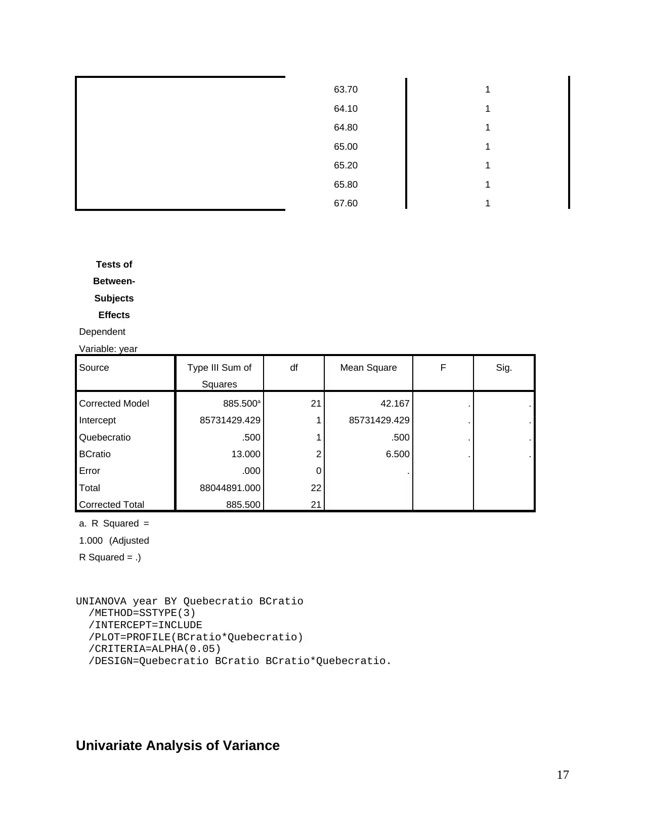
63.70 1
64.10 1
64.80 1
65.00 1
65.20 1
65.80 1
67.60 1
Tests of
Between-
Subjects
Effects
Dependent
Variable: year
Source Type III Sum of
Squares
df Mean Square F Sig.
Corrected Model 885.500a 21 42.167 . .
Intercept 85731429.429 1 85731429.429 . .
Quebecratio .500 1 .500 . .
BCratio 13.000 2 6.500 . .
Error .000 0 .
Total 88044891.000 22
Corrected Total 885.500 21
a. R Squared =
1.000 (Adjusted
R Squared = .)
UNIANOVA year BY Quebecratio BCratio
/METHOD=SSTYPE(3)
/INTERCEPT=INCLUDE
/PLOT=PROFILE(BCratio*Quebecratio)
/CRITERIA=ALPHA(0.05)
/DESIGN=Quebecratio BCratio BCratio*Quebecratio.
Univariate Analysis of Variance
17
Paraphrase This Document
Need a fresh take? Get an instant paraphrase of this document with our AI Paraphraser
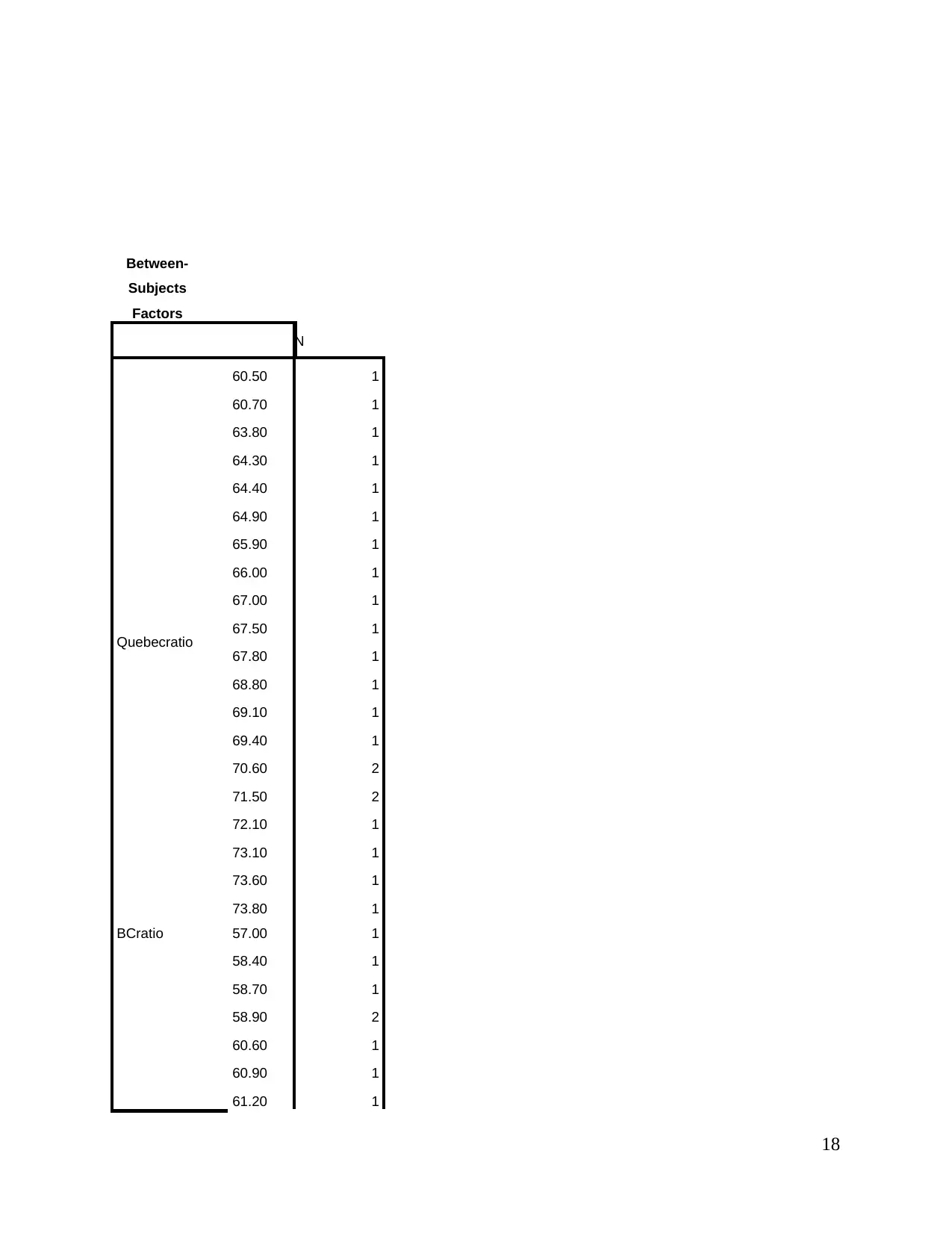
Between-
Subjects
Factors
N
Quebecratio
60.50 1
60.70 1
63.80 1
64.30 1
64.40 1
64.90 1
65.90 1
66.00 1
67.00 1
67.50 1
67.80 1
68.80 1
69.10 1
69.40 1
70.60 2
71.50 2
72.10 1
73.10 1
73.60 1
73.80 1
BCratio 57.00 1
58.40 1
58.70 1
58.90 2
60.60 1
60.90 1
61.20 1
18
Subjects
Factors
N
Quebecratio
60.50 1
60.70 1
63.80 1
64.30 1
64.40 1
64.90 1
65.90 1
66.00 1
67.00 1
67.50 1
67.80 1
68.80 1
69.10 1
69.40 1
70.60 2
71.50 2
72.10 1
73.10 1
73.60 1
73.80 1
BCratio 57.00 1
58.40 1
58.70 1
58.90 2
60.60 1
60.90 1
61.20 1
18
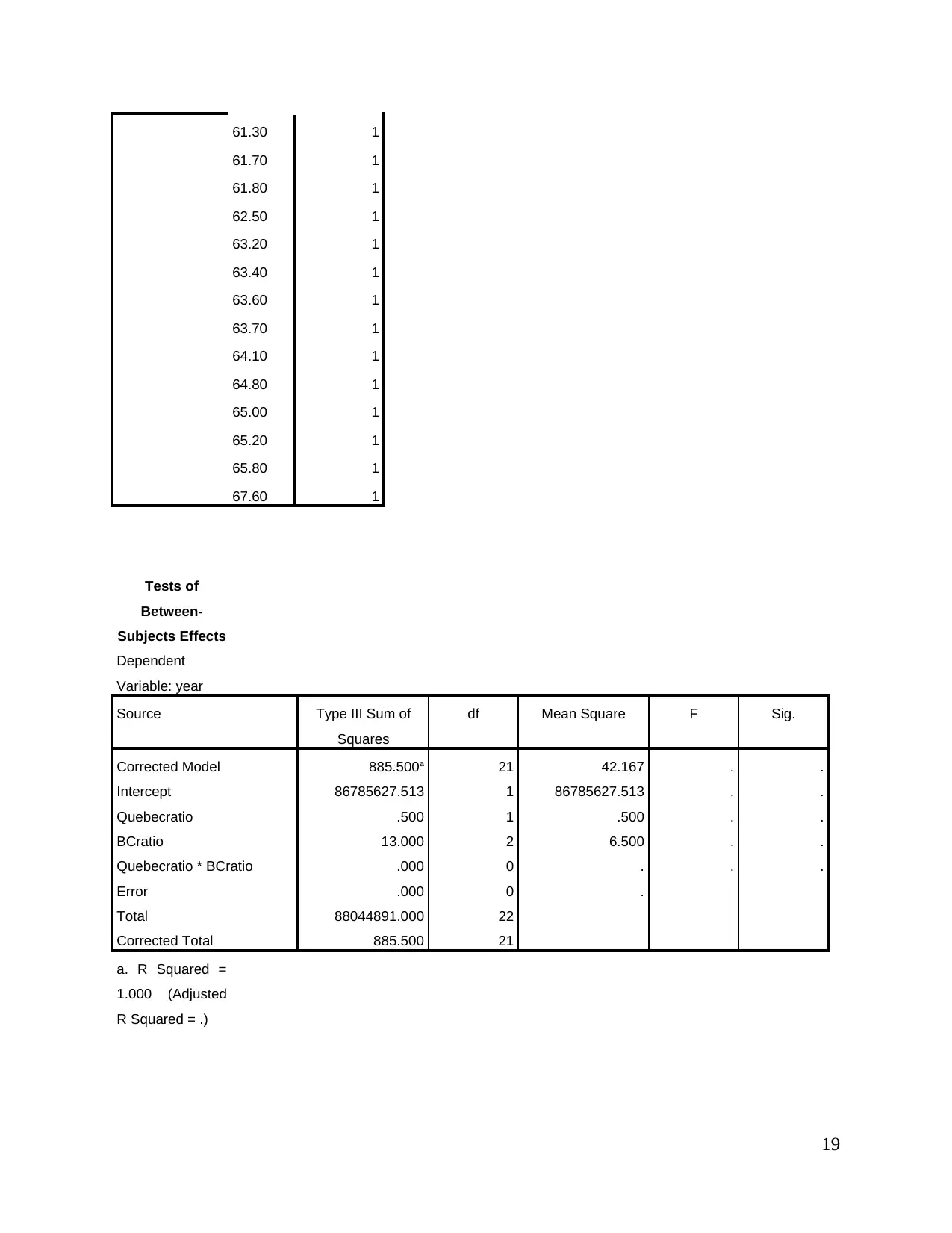
61.30 1
61.70 1
61.80 1
62.50 1
63.20 1
63.40 1
63.60 1
63.70 1
64.10 1
64.80 1
65.00 1
65.20 1
65.80 1
67.60 1
Tests of
Between-
Subjects Effects
Dependent
Variable: year
Source Type III Sum of
Squares
df Mean Square F Sig.
Corrected Model 885.500a 21 42.167 . .
Intercept 86785627.513 1 86785627.513 . .
Quebecratio .500 1 .500 . .
BCratio 13.000 2 6.500 . .
Quebecratio * BCratio .000 0 . . .
Error .000 0 .
Total 88044891.000 22
Corrected Total 885.500 21
a. R Squared =
1.000 (Adjusted
R Squared = .)
19
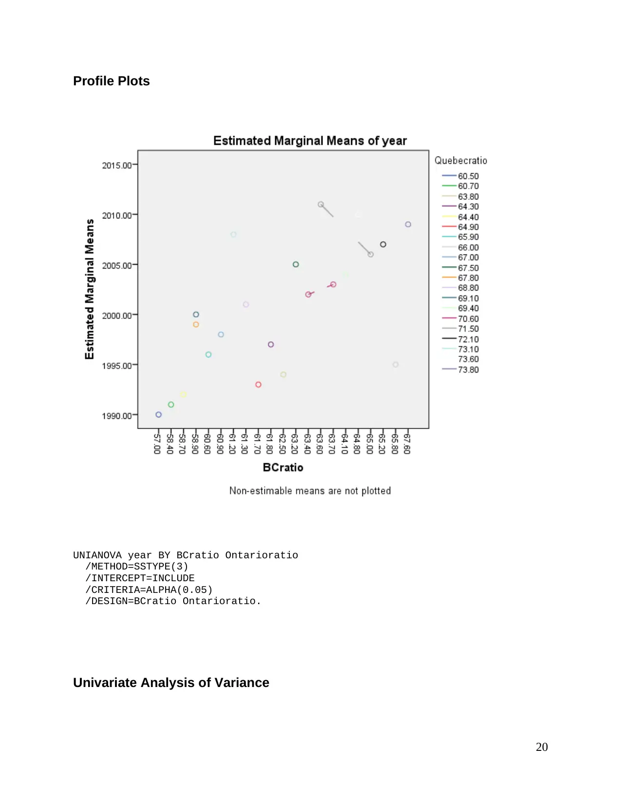
Profile Plots
UNIANOVA year BY BCratio Ontarioratio
/METHOD=SSTYPE(3)
/INTERCEPT=INCLUDE
/CRITERIA=ALPHA(0.05)
/DESIGN=BCratio Ontarioratio.
Univariate Analysis of Variance
20
UNIANOVA year BY BCratio Ontarioratio
/METHOD=SSTYPE(3)
/INTERCEPT=INCLUDE
/CRITERIA=ALPHA(0.05)
/DESIGN=BCratio Ontarioratio.
Univariate Analysis of Variance
20
Secure Best Marks with AI Grader
Need help grading? Try our AI Grader for instant feedback on your assignments.
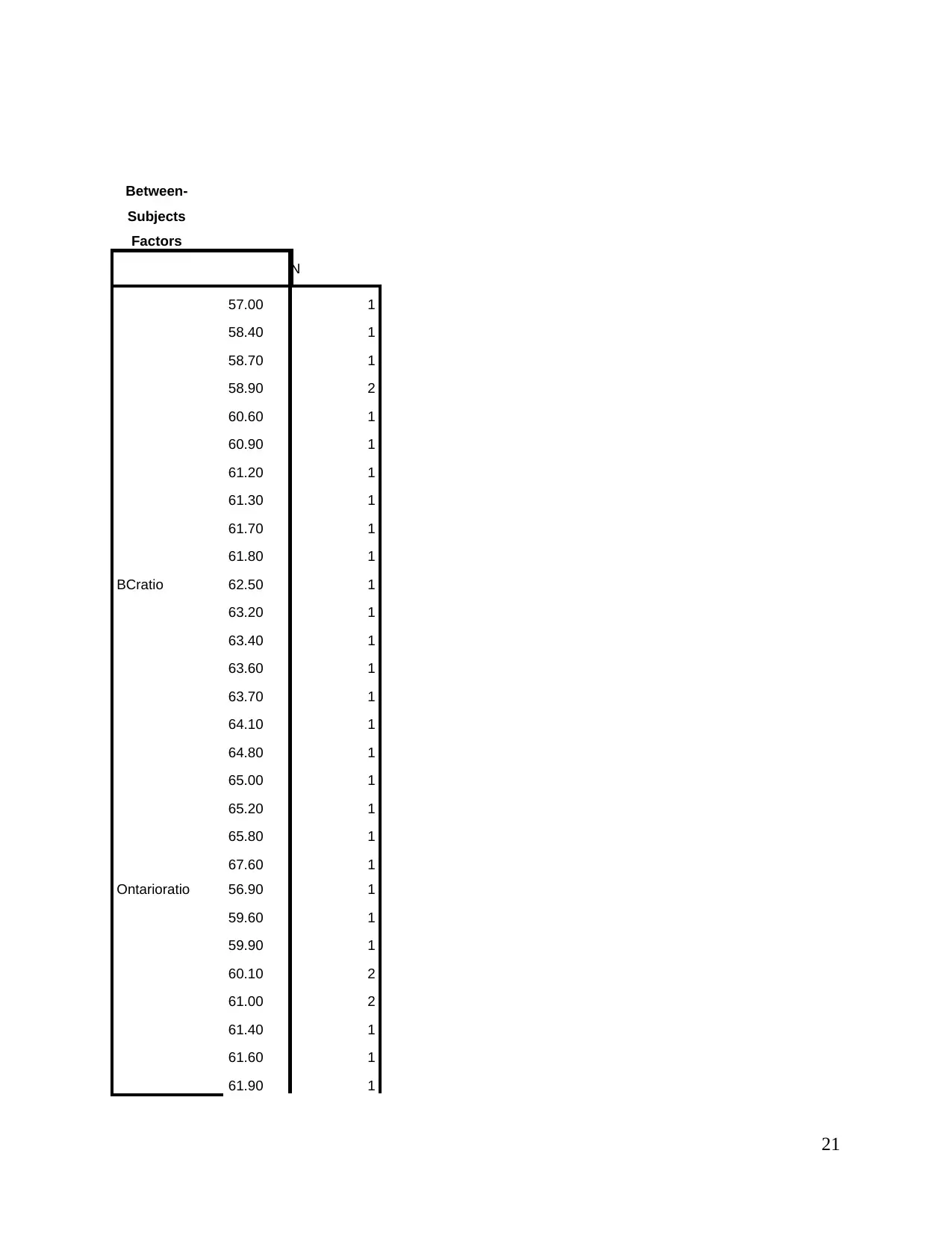
Between-
Subjects
Factors
N
BCratio
57.00 1
58.40 1
58.70 1
58.90 2
60.60 1
60.90 1
61.20 1
61.30 1
61.70 1
61.80 1
62.50 1
63.20 1
63.40 1
63.60 1
63.70 1
64.10 1
64.80 1
65.00 1
65.20 1
65.80 1
67.60 1
Ontarioratio 56.90 1
59.60 1
59.90 1
60.10 2
61.00 2
61.40 1
61.60 1
61.90 1
21
Subjects
Factors
N
BCratio
57.00 1
58.40 1
58.70 1
58.90 2
60.60 1
60.90 1
61.20 1
61.30 1
61.70 1
61.80 1
62.50 1
63.20 1
63.40 1
63.60 1
63.70 1
64.10 1
64.80 1
65.00 1
65.20 1
65.80 1
67.60 1
Ontarioratio 56.90 1
59.60 1
59.90 1
60.10 2
61.00 2
61.40 1
61.60 1
61.90 1
21
62.10 1
63.10 1
63.50 1
63.90 1
64.40 1
64.70 2
66.10 1
67.10 1
68.50 1
71.80 1
72.10 1
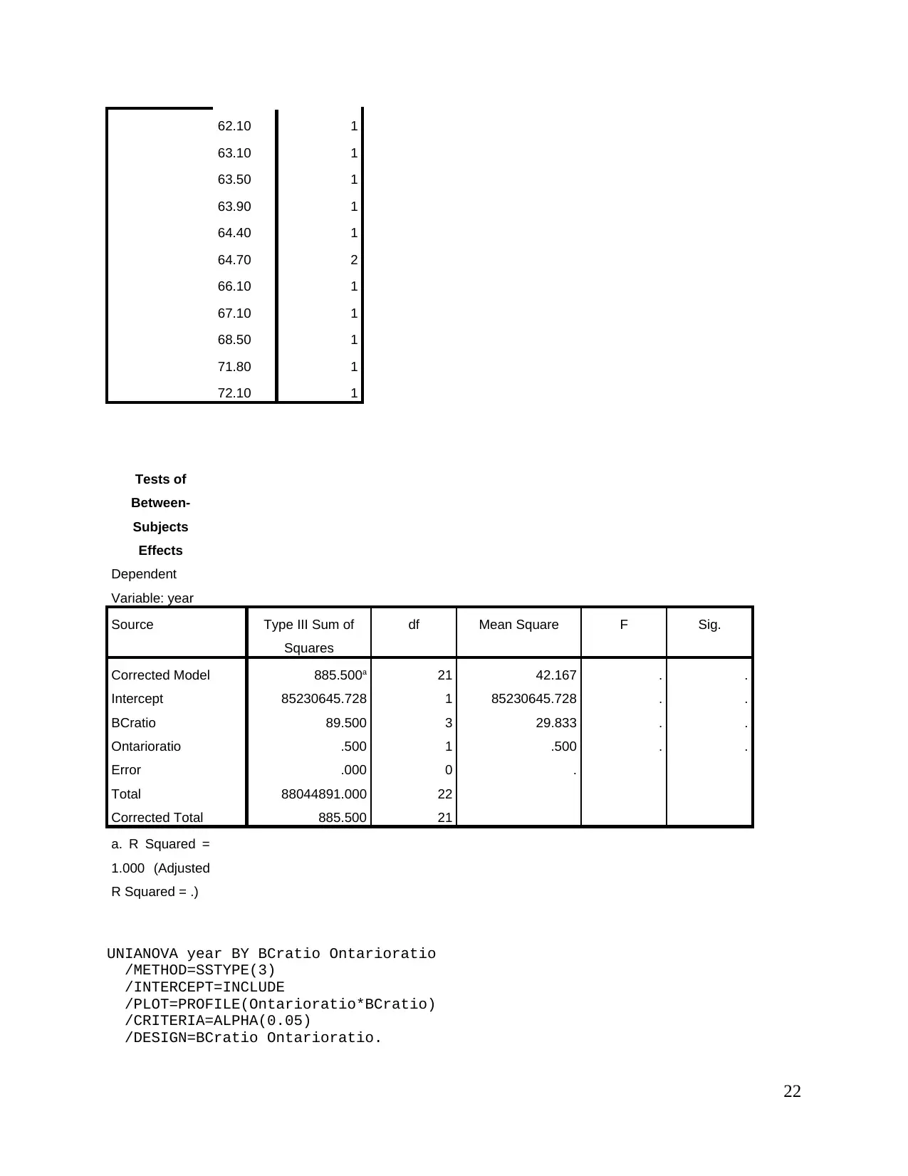
Tests of
Between-
Subjects
Effects
Dependent
Variable: year
Source Type III Sum of
Squares
df Mean Square F Sig.
Corrected Model 885.500a 21 42.167 . .
Intercept 85230645.728 1 85230645.728 . .
BCratio 89.500 3 29.833 . .
Ontarioratio .500 1 .500 . .
Error .000 0 .
Total 88044891.000 22
Corrected Total 885.500 21
a. R Squared =
1.000 (Adjusted
R Squared = .)
UNIANOVA year BY BCratio Ontarioratio
/METHOD=SSTYPE(3)
/INTERCEPT=INCLUDE
/PLOT=PROFILE(Ontarioratio*BCratio)
/CRITERIA=ALPHA(0.05)
/DESIGN=BCratio Ontarioratio.
22
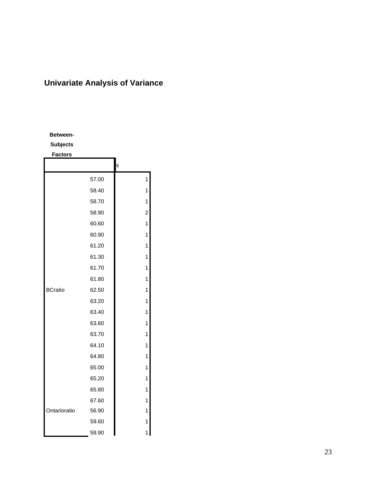
Univariate Analysis of Variance
Between-
Subjects
Factors
N
BCratio
57.00 1
58.40 1
58.70 1
58.90 2
60.60 1
60.90 1
61.20 1
61.30 1
61.70 1
61.80 1
62.50 1
63.20 1
63.40 1
63.60 1
63.70 1
64.10 1
64.80 1
65.00 1
65.20 1
65.80 1
67.60 1
Ontarioratio 56.90 1
59.60 1
59.90 1
23
Between-
Subjects
Factors
N
BCratio
57.00 1
58.40 1
58.70 1
58.90 2
60.60 1
60.90 1
61.20 1
61.30 1
61.70 1
61.80 1
62.50 1
63.20 1
63.40 1
63.60 1
63.70 1
64.10 1
64.80 1
65.00 1
65.20 1
65.80 1
67.60 1
Ontarioratio 56.90 1
59.60 1
59.90 1
23
Paraphrase This Document
Need a fresh take? Get an instant paraphrase of this document with our AI Paraphraser
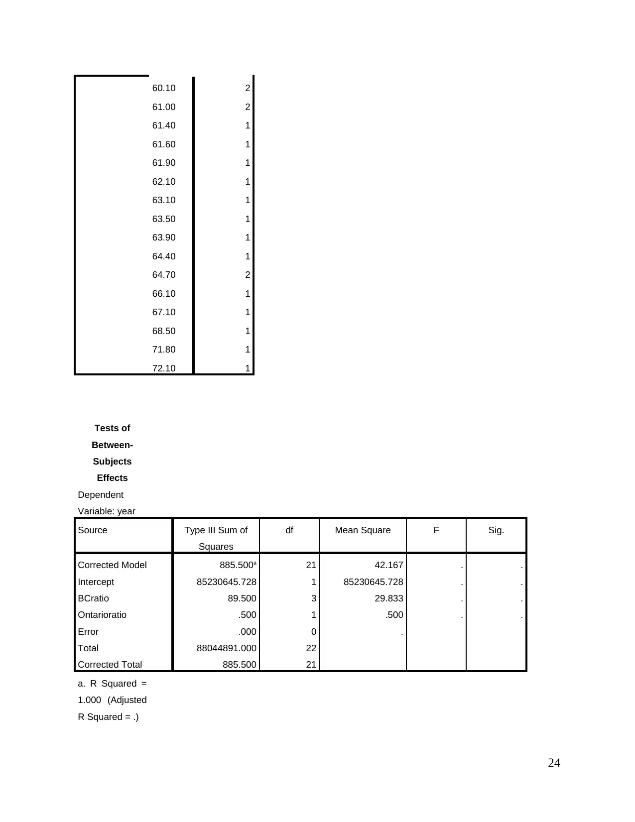
60.10 2
61.00 2
61.40 1
61.60 1
61.90 1
62.10 1
63.10 1
63.50 1
63.90 1
64.40 1
64.70 2
66.10 1
67.10 1
68.50 1
71.80 1
72.10 1
Tests of
Between-
Subjects
Effects
Dependent
Variable: year
Source Type III Sum of
Squares
df Mean Square F Sig.
Corrected Model 885.500a 21 42.167 . .
Intercept 85230645.728 1 85230645.728 . .
BCratio 89.500 3 29.833 . .
Ontarioratio .500 1 .500 . .
Error .000 0 .
Total 88044891.000 22
Corrected Total 885.500 21
a. R Squared =
1.000 (Adjusted
R Squared = .)
24
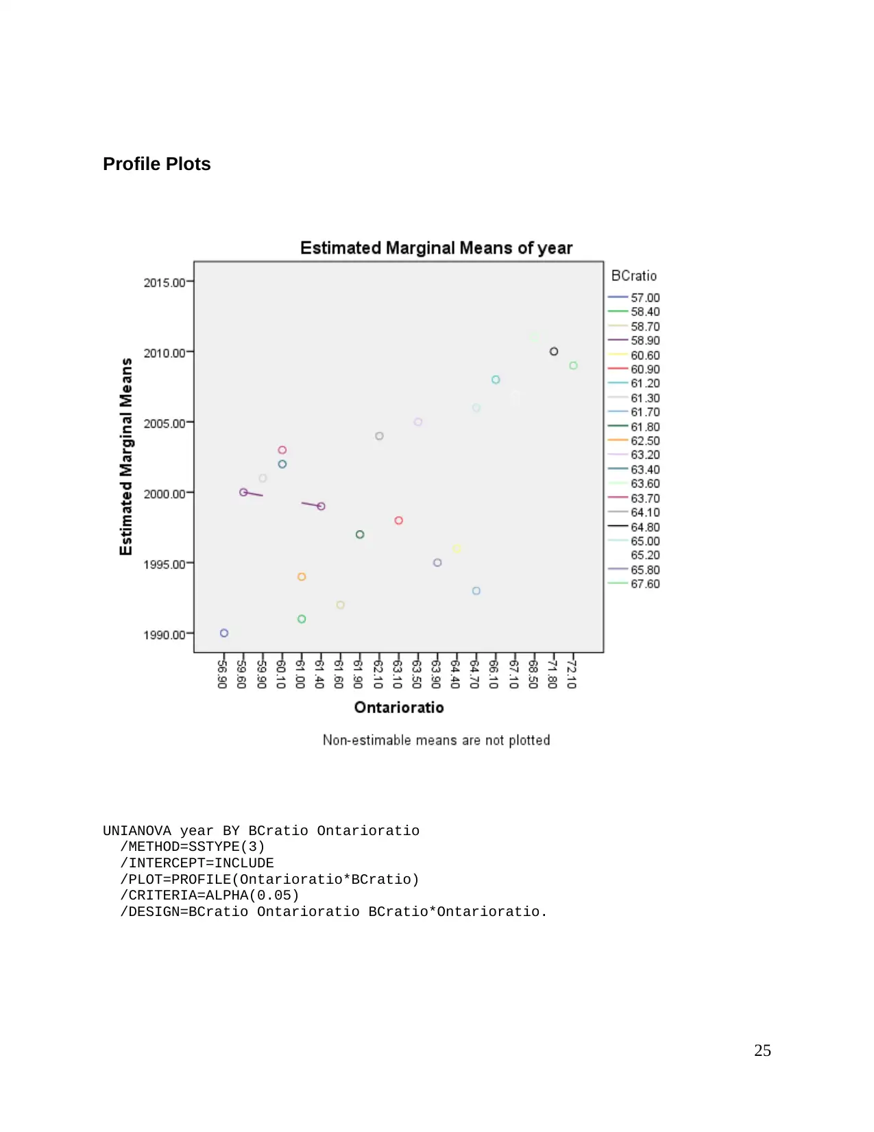
Profile Plots
UNIANOVA year BY BCratio Ontarioratio
/METHOD=SSTYPE(3)
/INTERCEPT=INCLUDE
/PLOT=PROFILE(Ontarioratio*BCratio)
/CRITERIA=ALPHA(0.05)
/DESIGN=BCratio Ontarioratio BCratio*Ontarioratio.
25
UNIANOVA year BY BCratio Ontarioratio
/METHOD=SSTYPE(3)
/INTERCEPT=INCLUDE
/PLOT=PROFILE(Ontarioratio*BCratio)
/CRITERIA=ALPHA(0.05)
/DESIGN=BCratio Ontarioratio BCratio*Ontarioratio.
25
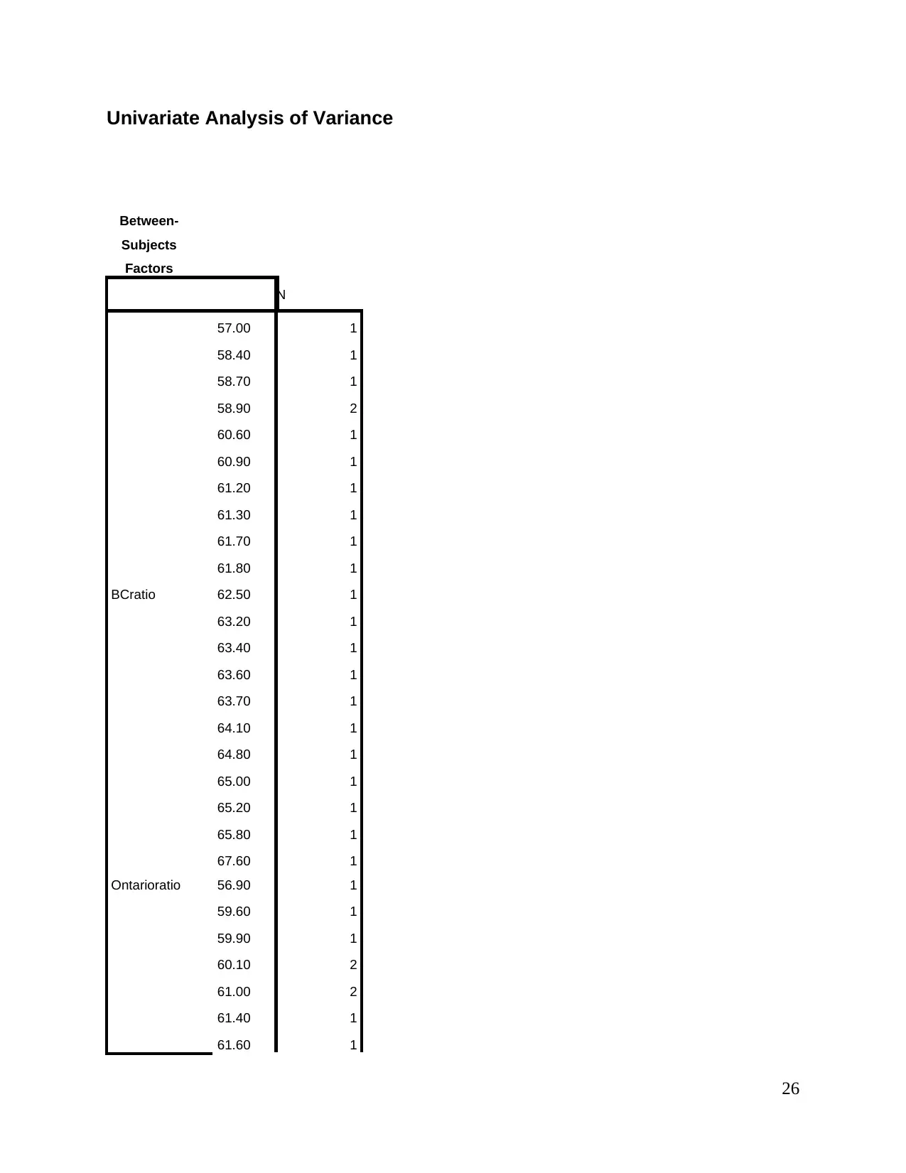
Univariate Analysis of Variance
Between-
Subjects
Factors
N
BCratio
57.00 1
58.40 1
58.70 1
58.90 2
60.60 1
60.90 1
61.20 1
61.30 1
61.70 1
61.80 1
62.50 1
63.20 1
63.40 1
63.60 1
63.70 1
64.10 1
64.80 1
65.00 1
65.20 1
65.80 1
67.60 1
Ontarioratio 56.90 1
59.60 1
59.90 1
60.10 2
61.00 2
61.40 1
61.60 1
26
Between-
Subjects
Factors
N
BCratio
57.00 1
58.40 1
58.70 1
58.90 2
60.60 1
60.90 1
61.20 1
61.30 1
61.70 1
61.80 1
62.50 1
63.20 1
63.40 1
63.60 1
63.70 1
64.10 1
64.80 1
65.00 1
65.20 1
65.80 1
67.60 1
Ontarioratio 56.90 1
59.60 1
59.90 1
60.10 2
61.00 2
61.40 1
61.60 1
26
Secure Best Marks with AI Grader
Need help grading? Try our AI Grader for instant feedback on your assignments.
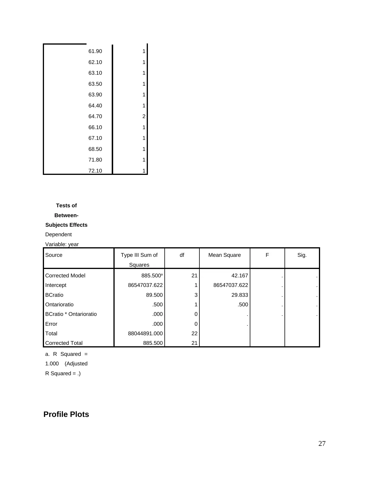
61.90 1
62.10 1
63.10 1
63.50 1
63.90 1
64.40 1
64.70 2
66.10 1
67.10 1
68.50 1
71.80 1
72.10 1
Tests of
Between-
Subjects Effects
Dependent
Variable: year
Source Type III Sum of
Squares
df Mean Square F Sig.
Corrected Model 885.500a 21 42.167 . .
Intercept 86547037.622 1 86547037.622 . .
BCratio 89.500 3 29.833 . .
Ontarioratio .500 1 .500 . .
BCratio * Ontarioratio .000 0 . . .
Error .000 0 .
Total 88044891.000 22
Corrected Total 885.500 21
a. R Squared =
1.000 (Adjusted
R Squared = .)
Profile Plots
27
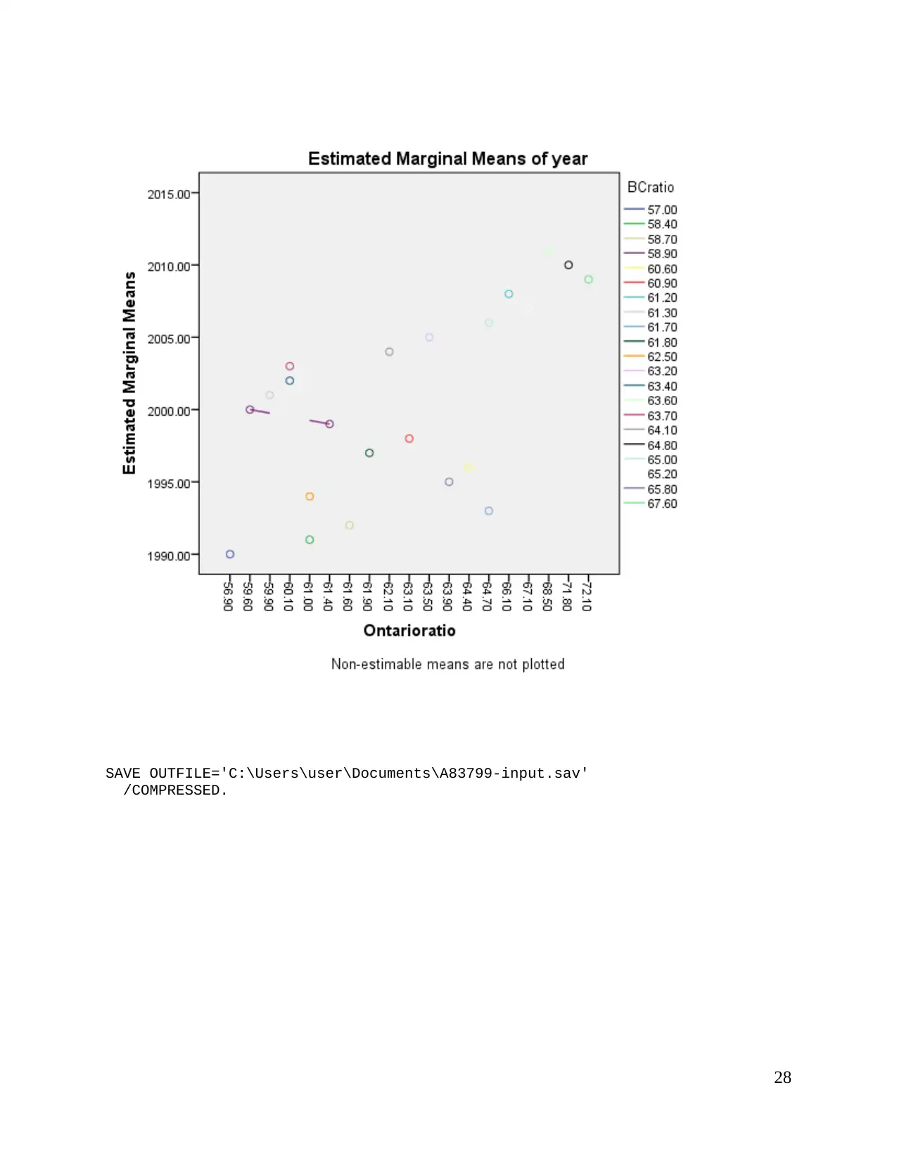
SAVE OUTFILE='C:\Users\user\Documents\A83799-input.sav'
/COMPRESSED.
28
/COMPRESSED.
28
1 out of 30
Related Documents
Your All-in-One AI-Powered Toolkit for Academic Success.
+13062052269
info@desklib.com
Available 24*7 on WhatsApp / Email
![[object Object]](/_next/static/media/star-bottom.7253800d.svg)
Unlock your academic potential
© 2024 | Zucol Services PVT LTD | All rights reserved.


