Linear Advection Equation - Accuracy, Stability, Convergence.

Accuracy, Stability, Convergence
Linear Advection Equation
Student Name –
Student ID –

Contents
Aim :..................................................................................................................... 3
Method :................................................................................................................ 3
Discussion :............................................................................................................ 3
Results :................................................................................................................. 6
Conclusion :........................................................................................................... 9
Appendix :............................................................................................................. 9
Aim :
The aim here is the study of the numerical solutions of the linear advection equation and to
study the accuracy, stability and convergence.

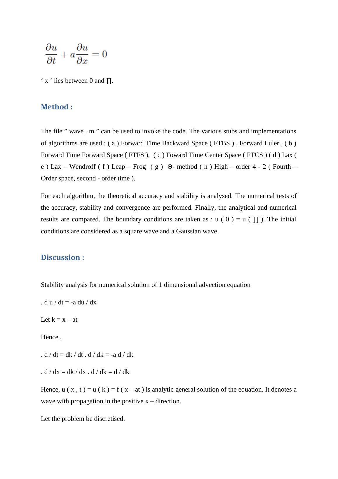
‘ x ’ lies between 0 and ∏.
Method :
The file ” wave . m ” can be used to invoke the code. The various stubs and implementations
of algorithms are used : ( a ) Forward Time Backward Space ( FTBS ) , Forward Euler , ( b )
Forward Time Forward Space ( FTFS ), ( c ) Foward Time Center Space ( FTCS ) ( d ) Lax (
e ) Lax – Wendroff ( f ) Leap – Frog ( g ) Θ- method ( h ) High – order 4 - 2 ( Fourth –
Order space, second - order time ).
For each algorithm, the theoretical accuracy and stability is analysed. The numerical tests of
the accuracy, stability and convergence are performed. Finally, the analytical and numerical
results are compared. The boundary conditions are taken as : u ( 0 ) = u ( ∏ ). The initial
conditions are considered as a square wave and a Gaussian wave.
Discussion :
Stability analysis for numerical solution of 1 dimensional advection equation
. d u / dt = -a du / dx
Let k = x – at
Hence ,
. d / dt = dk / dt . d / dk = -a d / dk
. d / dx = dk / dx . d / dk = d / dk
Hence, u ( x , t ) = u ( k ) = f ( x – at ) is analytic general solution of the equation. It denotes a
wave with propagation in the positive x – direction.
Let the problem be discretised.

Also, xi = x0 + i ∆x , i = 0 , 1 , ...... , n + 1
And tj = t0 + j ∆t , j = 0 , ......., m
U i j = u ( xi , tj )
The single eigen mode U i j depends on ‘ t ’ by powers of k ( k j ).
U t = - a U x has an exact solution given by u ( x , t ) = e i ( px + wt ) using Fourier analysis.
The dispersion relation is given by w = - a . p
Hence, u ( x , t ) = e i p ( x - at ) = f ( x – at )
There is no damping and the amplitude remains constant and dispersion is absent if the time
step is chosen such that the dispersion relation mentioned above holds good. But if some
other ‘t’ step is used, then dispersion may be present.
The dispersion relation will be satisfied in case ∆ t = ∆ x / a
. as k j = e – i p ∆ x
U i j = k j e i p i ∆ x
U i j = e i p ( - j ∆ x + i ∆ x )
Let x i = i ∆ x, t j = j ∆ t
∆ x = ∆ t . a
U i j = e i p ( - a j ∆ t + i ∆ x ) = e – i p ( x i – a t j ) = f ( x i – a t j )
This is the exact solution. Hence, no dispersion is present.
Solution of 1 dimensional linear advection equation :
Ut + a Ux = 0
If initially ( x , t ) = ( x0 , 0 )
. dx / dh = a
 X = ah + c1
 . x ( 0 ) = x0 = c1

 => x = c1 . h + x0
 Dt / dh = 1 and t = h + c2
Also, t ( 0 ) = 0 = c2
Hence, t = h
So, x = at + x0
Solving for U :
. dU / dh = dt / dh Ut + dx / dh Ux = Ut + a Ux = 0
. dU / dh = 0
 U = c3
 Hence, U is constant for the characteristic curves.
U ( h = 0 , x0 ) = f ( x0 ) = c3
U = f ( x0 ) = f ( x – at )
Since, x0 = x – at
The solution is similar to the D’Alembert’s solution obtained for a wave which moves
towards right with a speed ‘a’.
Equation of the characteristic curve :
X = x + at
. t = 1 / a ( x – x0 )
The slope and ‘u’ are constant for the curves. If the 1 dimensional advection equation is
solved using finite difference having initial condition of a Gaussian pulse, then dispersion
gets introduced due to varying speed of wave. But the spectral method gives better results.
If the 1 dimensional advection equation is solved using spectral method having initial
condition of a square wave, then dispersion gets introduced due to varying speed of wave.
But the finite difference method gives better results.
In spectral method, for approximation of initial conditions, Fourier series is used, which does
not work accurately. In the finite difference method, dispersion can be chosen using the
condition ∆ t = ∆ x / a.
Stability :
( a )
Analysis of FTBS

FTBS is accurate in both the first order space and time. It is stable conditionally for Courant
number between 0 and 1.
Case : Square wave
If Courant number = 1, the system was stable with no error. If the Courant number is greater
than 1, unstable results are obtained.
If the Courant number is 0 < CN < 1, the solution smooths out fastly.
If the Courant number < 0, then the behaviour is similar to the one when value > 1 and does
not depend on the number of grid points.
Forward Time Backward Space ( FTBS ) , Forward Euler,
The FTBS method gives
U i j + 1 = U i j - a ∆t / 2 ∆x [ U i + 1 j - U i – 1 j ]
FTBS is found to be unstable.
If the eigen modes or independent solutions of the above equation are represented by
U i j = k j e i ( p i ∆ x )
Here, p = real spatial wave number and k is a complex number.
If | k ( p ) | > 1 for some value of ‘ p ’, then the equation becomes unstable.
( b ) Analysis of Lax – Wendroff
The Fourier Transform can be used for converting the discrete finite difference to wave space
solution. The Courant number and the algorithm decide how the amplitude increases or
decreases. The growing waves show instability and the decaying waves show stability.
Lax – Wendroff is accurate in both the first order space and time. It is also stable conditionally for
Courant number between 0 and 1.
Case : Square wave
If Courant number = 1, the system was stable with some error. If the Courant number is
greater than 1, unstable results are obtained.
If the Courant number is 0 < CN < 1, the solution smooths out slowly.