ACFI7027 Quantitative Methods for Finance

This document includes tasks related to multicollinearity, simple linear regression, improving the quality of the model, stationarity and its importance in time series analysis, calculation of present value of series of payments made to the bond holder, determination of the date of first coupon payment, purpose of discounting future cash flows and determination of appropriate discounting rate, and determination of a formula for total revenue from producing and selling quantities Q1 and Q2. The subject is ACFI7027 Quantitative Methods for Finance.

ACFI7027 QUANTITATIVE
METHODS FOR FINANCE

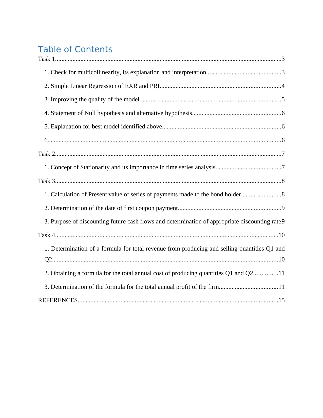
Table of Contents
Task 1...............................................................................................................................................3
1. Check for multicollinearity, its explanation and interpretation...............................................3
2. Simple Linear Regression of EXR and PRI............................................................................4
3. Improving the quality of the model.........................................................................................5
4. Statement of Null hypothesis and alternative hypothesis........................................................6
5. Explanation for best model identified above...........................................................................6
6...................................................................................................................................................6
Task 2...............................................................................................................................................7
1. Concept of Stationarity and its importance in time series analysis.........................................7
Task 3...............................................................................................................................................8
1. Calculation of Present value of series of payments made to the bond holder.........................8
2. Determination of the date of first coupon payment.................................................................9
3. Purpose of discounting future cash flows and determination of appropriate discounting rate9
Task 4.............................................................................................................................................10
1. Determination of a formula for total revenue from producing and selling quantities Q1 and
Q2..............................................................................................................................................10
2. Obtaining a formula for the total annual cost of producing quantities Q1 and Q2...............11
3. Determination of the formula for the total annual profit of the firm.....................................11
REFERENCES..............................................................................................................................15

Task 1
1. Check for multicollinearity, its explanation and interpretation
Multicollinearity that could be checked through regression analysis technique occurs
when high degree of correlation exists among independent variables which leads to non-
provision of any independent or unique information through regression model (Harvey, Liu and
Saretto, 2020). Also, a very high degree of correlation existing among variables leads to
problems in terms of fitting and interpreting the regression model. In order to detect
multicollinearity, a metric known as Variance Inflation Index VIF is used which helps in
identifying or measuring the strength of correlation and correlation among independent variables
included in the regression model.
Coefficientsa
Model Unstandardize
d Coefficients
Standardize
d
Coefficients
t Sig. Collinearity
Statistics
B Std.
Error
Beta Toleranc
e
VIF
1 (Constant) 1.536 .810 1.89
5
.07
0
Interest Rate -.004 .023 -.152 -.165 .87
0
.032 30.91
9
Consumer
Price Index
.000 .004 -.099 -.115 .91
0
.037 27.34
7
Inflation Rate -.017 .014 -.394 -
1.21
1
.23
8
.259 3.854
Unemploymen
t Rate
-.011 .012 -.288 -.933 .36
0
.289 3.465
Industrial
Production
Index
-.007 .005 -.530 -
1.56
2
.13
1
.238 4.194
a. Dependent Variable: Exchange Rate
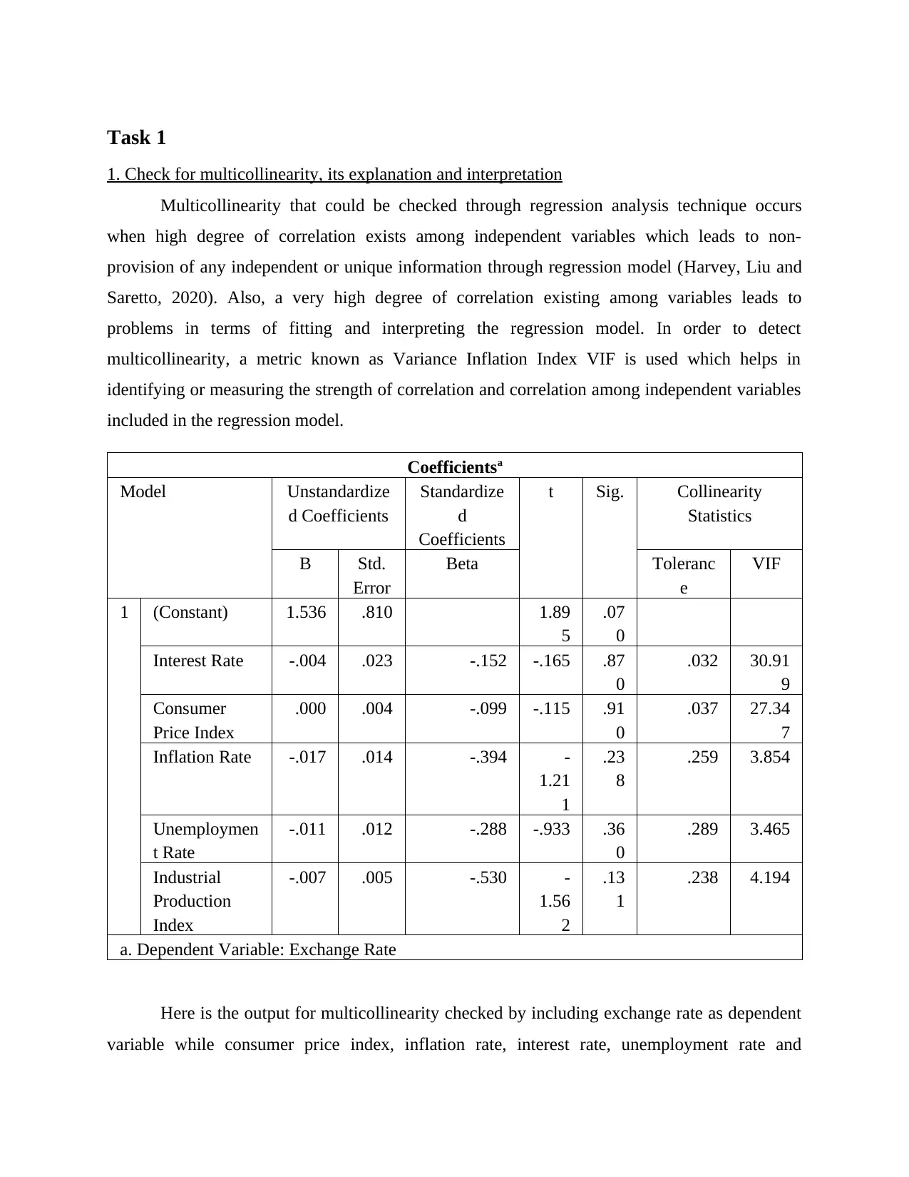
Here is the output for multicollinearity checked by including exchange rate as dependent
variable while consumer price index, inflation rate, interest rate, unemployment rate and

industrial production index are included as independent variables by ensuring that the five
independent variables are not highly correlated with each other. For this, VIF values for each of
the predictor variable has been obtained in order to determine the multicollinearity. The VIF
values have lower limit as 1 while having no upper limit Accordingly, the VIF values for each of
the predictor variable has been obtained as follows:
Interest rate = 30.919
Consumer Price Index = 27.347
Inflation rate = 3.854
Unemployment rate = 3.465
Industrial production index = 4.194
From the above results obtained in terms of VIF values, it can be found that none of the
predictor variable is having 1 as a VIF value while there are predictor variables that is, inflation
rate, unemployment rate and industrial production index where VIF values fall in the range of 1
and 5 which indicates presence of moderate correlation among one predictor variable to other
predictor variables involves in the model (James, 2020). However, a very high value of VIF for
interest rate and consumer price index shows there exists severe correlation between a particular
predictor variable and other predictor variables in the model. Accordingly, multicollinearity
would be a problem in this particular regression model and to avoid this problem such high
correlated independent variables should be removed from the model.
2. Simple Linear Regression of EXR and PRI
Model Summary
Mode
l
R R
Squar
e
Adjuste
d R
Square
Std.
Error of
the
Estimat
e
Change Statistics
R
Square
Chang
e
F
Chang
e
df
1
df
2
Sig. F
Chang
e
1 .559
a
.313 .289 .06207 .313 13.201 1 29 .001
a. Predictors: (Constant), Consumer Price Index

ANOVAa
Model Sum of
Squares
df Mean
Square
F Sig.
1 Regressio
n
.051 1 .051 13.201 .001b
Residual .112 29 .004
Total .163 30
a. Dependent Variable: Exchange Rate
b. Predictors: (Constant), Consumer Price Index
Coefficientsa
Model Unstandardized
Coefficients
Standardize
d
Coefficients
t Sig.
B Std. Error Beta
1 (Constant) .420 .060 6.938 .000
Consumer Price
Index
.002 .001 .559 3.633 .001
a. Dependent Variable: Exchange Rate
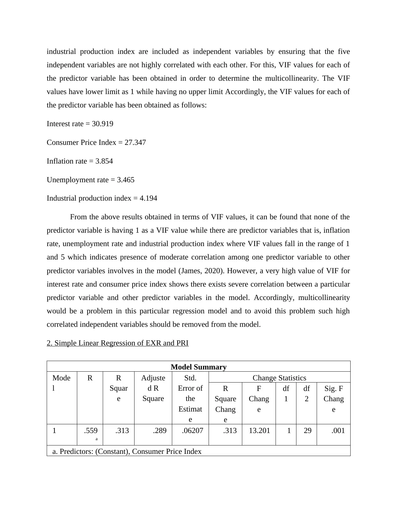
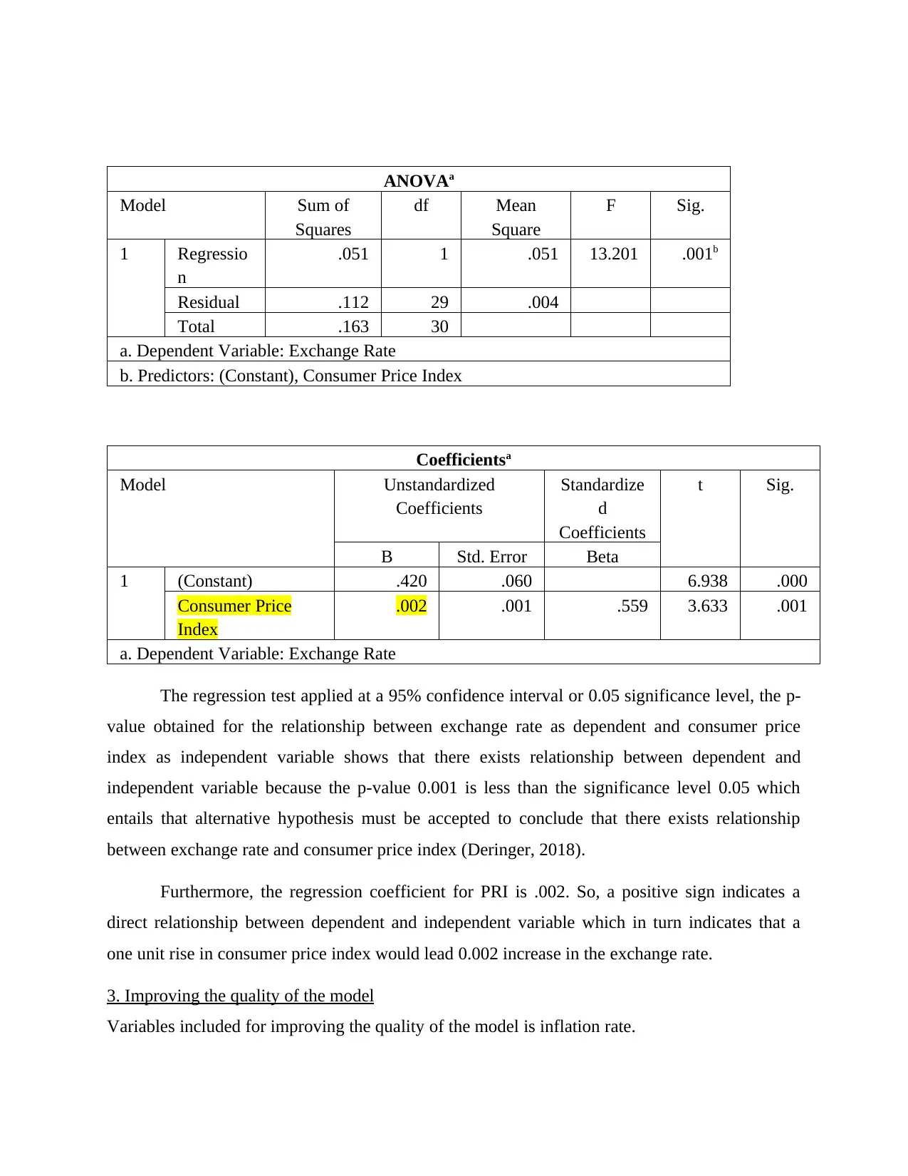
The regression test applied at a 95% confidence interval or 0.05 significance level, the p-
value obtained for the relationship between exchange rate as dependent and consumer price
index as independent variable shows that there exists relationship between dependent and
independent variable because the p-value 0.001 is less than the significance level 0.05 which
entails that alternative hypothesis must be accepted to conclude that there exists relationship
between exchange rate and consumer price index (Deringer, 2018).
Furthermore, the regression coefficient for PRI is .002. So, a positive sign indicates a
direct relationship between dependent and independent variable which in turn indicates that a
one unit rise in consumer price index would lead 0.002 increase in the exchange rate.
3. Improving the quality of the model
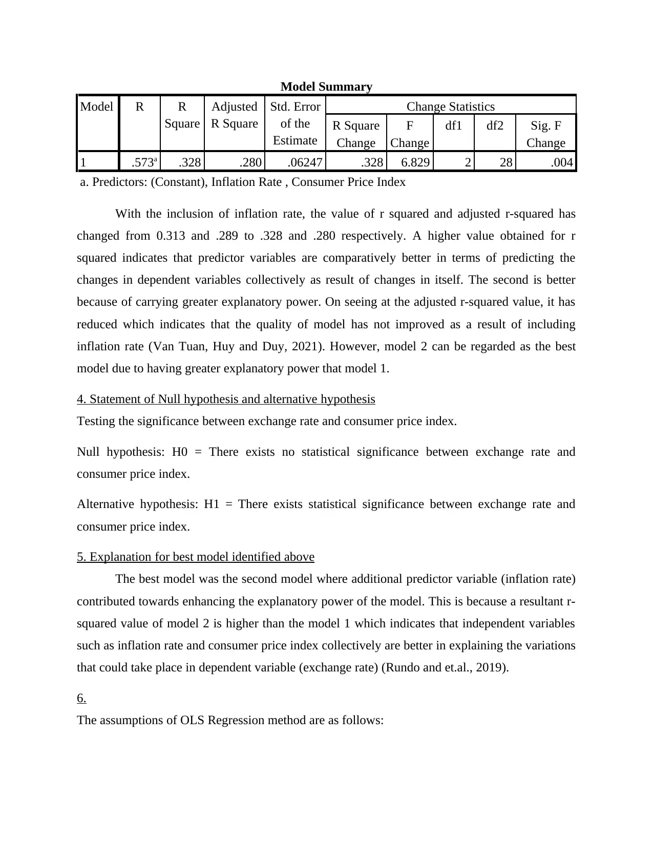
Variables included for improving the quality of the model is inflation rate.

Model Summary
Model R R
Square
Adjusted
R Square
Std. Error
of the
Estimate
Change Statistics
R Square
Change
F
Change
df1 df2 Sig. F
Change
1 .573a .328 .280 .06247 .328 6.829 2 28 .004
a. Predictors: (Constant), Inflation Rate , Consumer Price Index
With the inclusion of inflation rate, the value of r squared and adjusted r-squared has
changed from 0.313 and .289 to .328 and .280 respectively. A higher value obtained for r
squared indicates that predictor variables are comparatively better in terms of predicting the
changes in dependent variables collectively as result of changes in itself. The second is better
because of carrying greater explanatory power. On seeing at the adjusted r-squared value, it has
reduced which indicates that the quality of model has not improved as a result of including
inflation rate (Van Tuan, Huy and Duy, 2021). However, model 2 can be regarded as the best
model due to having greater explanatory power that model 1.
4. Statement of Null hypothesis and alternative hypothesis
Testing the significance between exchange rate and consumer price index.
Null hypothesis: H0 = There exists no statistical significance between exchange rate and
consumer price index.
Alternative hypothesis: H1 = There exists statistical significance between exchange rate and
consumer price index.
5. Explanation for best model identified above
The best model was the second model where additional predictor variable (inflation rate)
contributed towards enhancing the explanatory power of the model. This is because a resultant r-
squared value of model 2 is higher than the model 1 which indicates that independent variables
such as inflation rate and consumer price index collectively are better in explaining the variations
that could take place in dependent variable (exchange rate) (Rundo and et.al., 2019).
6.
The assumptions of OLS Regression method are as follows:

 Errors are normally distributed: In order to check or test whether this particular
assumption is violated or not in the OLS regression model, the implicit factor need to be
check. It means if there is lack of independence within a sample and show apparent non-
normality by a few point indicate that the assumption of normality is violated. This affect
the p values which is used for significant testing (Bagheri Bodaghabadi, 2018). However,
this assumption violation does not contribute to bias and inefficiency in regression model
 Homoscedasticity of errors: In case, if the graph shows the funnel shape to scattered plot
that this means that the assumption of homoscedasticity of errors are violated. The
homoscedasticity of error assumption indicates that across all the values of independent
variables, the variance of error term is similar. The impact of the violation of this
assumption on conclusion is that it makes coefficient less accurate. However, on the other
hand, this does not enhance the bias in the coefficient (Yang, Tu and Chen, 2019). The
assumption violation means the situation where assumption attached to specific statistical
procedure are not fulfilled. This affect the regression model with incorrect and
misleading results.
 Errors are not serially correlated: This is another assumption of OLS regression method
which indicate that error term for different time periods are not correlated. In order to
check whether the errors are serially correlated or not, the Durbin Watson (DW) test need
to apply. This test is used for identifying the autocorrelation which value ranging between
1 to 4. With the help of this test, if the value of DW test come between 2 to 4 that it
means that the assumptions are not violated as it indicates no serially correlation (Das,
2019). But in case of value come below 2 to 0, this means the assumption of errors are
not serially correlated is violate. The impact of which misleading conclusion will be
drawn.
Task 2
1. Concept of Stationarity and its importance in time series analysis
Stationarity refers to the statistical properties of the time series that is deemed to be not changing
over the time. Accordingly, a time series is deemed to be having stationarity when the shifts or
changes in time doesn’t cause changes in the shape of distribution (Rundo and et.al., 2019). The
reason for which stationarity important in time series is its usefulness at the time of applying

several analytical tools & models and tests in statistics which relies on it. Furthermore, it is
important because it helps in estimating parameters of a time series whose properties are not
going to change over the time in an easier and accurate manner. If the variance and mean of a
given time series keeps on changing over the time, there would be direct impact over the
accuracy of a time series over the time as well. Therefore, a time series that are affected by
trends or seasonality are not considered to be stationary as it affects the values with the series
over the time which in turn affects the value of its mean and variances.
2. In statistics, Dickey Fuller test is useful in testing the null hypothesis which indicates the
presence of unit root in an autoregressive model of time series. For the purpose of forecasting
and in order to ensure better prediction, stationary time series are used. To test the stationary,
Dicky Fuller test is being performed (Metu and Nwogwugwu, 2022). A unit root test is applied
to determine whether the time series is stationary or not which indicates the presence or absence
of unit root within the time series. When unit root is present, it defines that the null hypothesis
must be accepted for indicating the absence of stationarity while the alternative hypothesis is
meant for defining that the time series is stationary. In this way, Dicky Fuller test is useful in
determining whether the data series is stationary or not.
3. Augmented Dickey Fuller Test is known as the common statistical test meant for testing the
stationarity of time series which in turn gives results as the time series is stationary or not. Thus,
analysis of stationarity in time series is possible through Augmented Dickey Fuller Test. Dickey
Fuller test involves unit root testing for determining the presence or absence of stationarity with
the time series (Emerson and et.al., 2019). Unit roots are deemed to be causing unpredictable
results at the time of analyzing time series. However, Augmented Dickey Fuller test are used
with serial correlation meant for giving results indicating better prediction for the future.
Furthermore, Augmented Dickey Fuller Test is able to handle more complex models of time
series as compared to Dickey Fuller test, thus the former is considered to be more powerful than
the latter. In this way, ADF is utilized when the time series models are larger and complicated.
At last, the ADF statistic used in ADF test is a negative number and accordingly, when the
statistic is negative, there would be stronger rejection of the hypothesis that states that unit root is
present.

Task 3
1. Calculation of Present value of series of payments made to the bond holder
Formula for the sum of geometric progression for the finite terms is as follows:
P = A / r * [1 – 1 / (1 + r) n]
In the given case, the value of r 5.75% (coupon or fixed interest rate), n as 13 (the remaining
coupon payment from June 2023 to June 2035). Furthermore, the value of A is £5.75 (100 *
5.75%). There as the present value of the corporate bond as at 21st June 2022 could be
determined as follows with the help of above formula:
P = 5.75 / 0.0575 * [1 – 1 / (1 + 0.0575) 13]
P = 100 * [1 – 1 / 2.068]
P = 100 * [1 – 0.484]
P = 100 * 0.516
P = 51.6
Thus, the value of bond at 21st June 2022 would be £51.6.
2. Determination of the date of first coupon payment
To determine the date for the first coupon payment from 21st June 2022 where the present
value of this payment is less than £4.00, the value of n has been determined as follows:
First of all, discounting factor 65 periods or days have been determined and multiplied it with the
nominal value of bond that is, 100 which gives us the present value of coupon payment for 65
periods or days from now (21st June 2022). Accordingly, it has been identified that the present
value of coupon payment for the 58th day and onwards are found to be less than £4.00. Therefore,
the first payment would be done at 58th day from 21st June 2022 and the date for the first coupon
payment would be 18th August 2022.
3. Purpose of discounting future cash flows and determination of appropriate discounting rate
Future cash flows are discounted at the discounting rate in order to determine the present
value of cash flows where there lies an inverse relationship between discounting rate and present
value of cash flows because the latter gets reduced when the former is higher and also the present

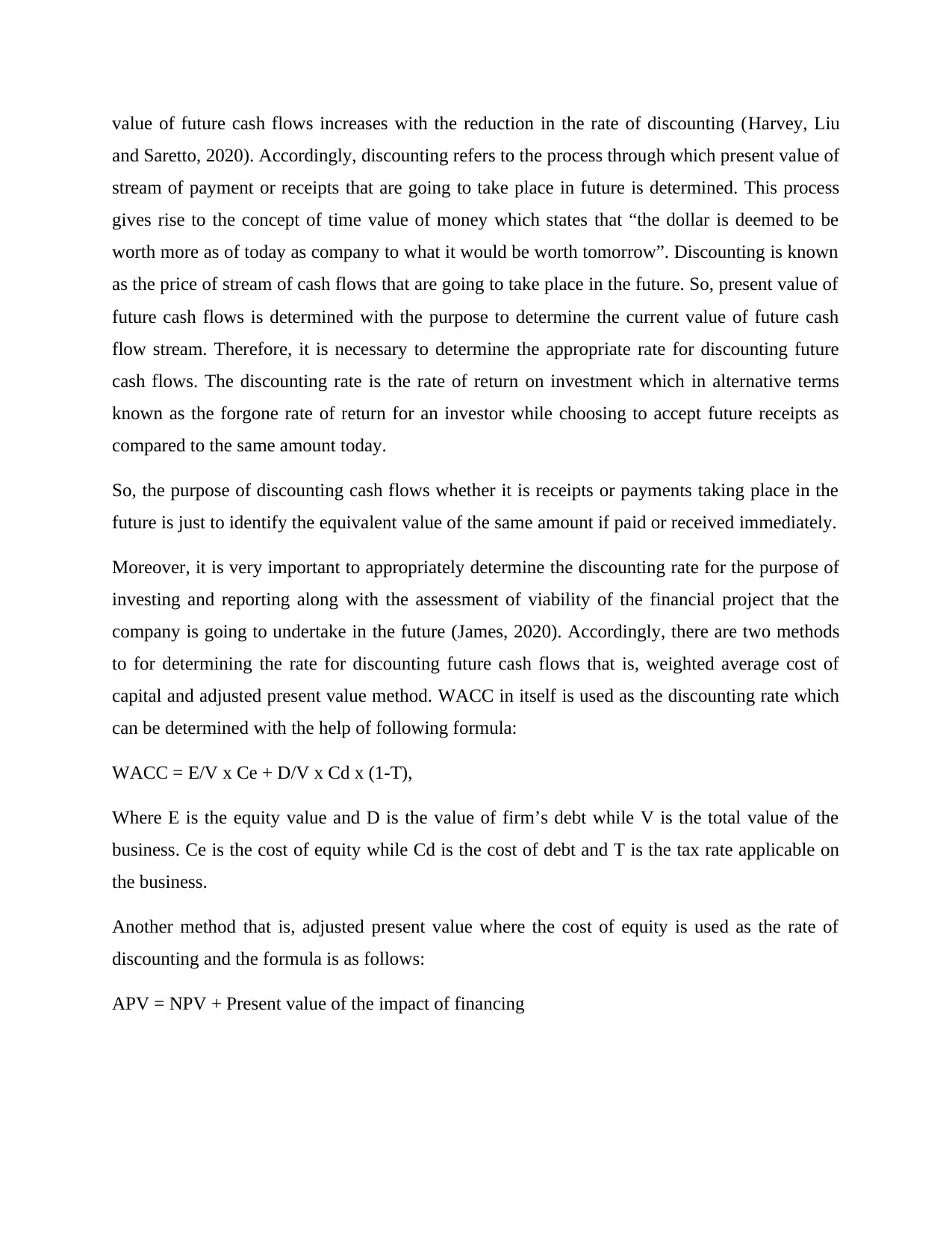
value of future cash flows increases with the reduction in the rate of discounting (Harvey, Liu
and Saretto, 2020). Accordingly, discounting refers to the process through which present value of
stream of payment or receipts that are going to take place in future is determined. This process
gives rise to the concept of time value of money which states that “the dollar is deemed to be
worth more as of today as company to what it would be worth tomorrow”. Discounting is known
as the price of stream of cash flows that are going to take place in the future. So, present value of
future cash flows is determined with the purpose to determine the current value of future cash
flow stream. Therefore, it is necessary to determine the appropriate rate for discounting future
cash flows. The discounting rate is the rate of return on investment which in alternative terms
known as the forgone rate of return for an investor while choosing to accept future receipts as
compared to the same amount today.
So, the purpose of discounting cash flows whether it is receipts or payments taking place in the
future is just to identify the equivalent value of the same amount if paid or received immediately.
Moreover, it is very important to appropriately determine the discounting rate for the purpose of
investing and reporting along with the assessment of viability of the financial project that the
company is going to undertake in the future (James, 2020). Accordingly, there are two methods
to for determining the rate for discounting future cash flows that is, weighted average cost of
capital and adjusted present value method. WACC in itself is used as the discounting rate which
can be determined with the help of following formula:
WACC = E/V x Ce + D/V x Cd x (1-T),
Where E is the equity value and D is the value of firm’s debt while V is the total value of the
business. Ce is the cost of equity while Cd is the cost of debt and T is the tax rate applicable on
the business.
Another method that is, adjusted present value where the cost of equity is used as the rate of
discounting and the formula is as follows:
APV = NPV + Present value of the impact of financing

Task 4
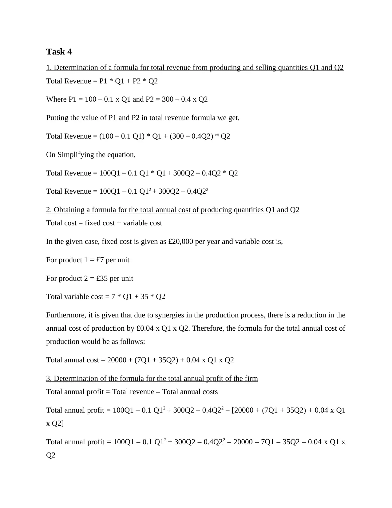
1. Determination of a formula for total revenue from producing and selling quantities Q1 and Q2
Total Revenue = P1 * Q1 + P2 * Q2
Where P1 = 100 – 0.1 x Q1 and P2 = 300 – 0.4 x Q2
Putting the value of P1 and P2 in total revenue formula we get,
Total Revenue = (100 – 0.1 Q1) * Q1 + (300 – 0.4Q2) * Q2
On Simplifying the equation,
Total Revenue = 100Q1 – 0.1 Q1 * Q1 + 300Q2 – 0.4Q2 * Q2
Total Revenue = 100Q1 – 0.1 Q12 + 300Q2 – 0.4Q22
2. Obtaining a formula for the total annual cost of producing quantities Q1 and Q2
Total cost = fixed cost + variable cost
In the given case, fixed cost is given as £20,000 per year and variable cost is,
For product 1 = £7 per unit
For product 2 = £35 per unit
Total variable cost = 7 * Q1 + 35 * Q2
Furthermore, it is given that due to synergies in the production process, there is a reduction in the
annual cost of production by £0.04 x Q1 x Q2. Therefore, the formula for the total annual cost of
production would be as follows:
Total annual cost = 20000 + (7Q1 + 35Q2) + 0.04 x Q1 x Q2
3. Determination of the formula for the total annual profit of the firm
Total annual profit = Total revenue – Total annual costs
Total annual profit = 100Q1 – 0.1 Q12 + 300Q2 – 0.4Q22 – [20000 + (7Q1 + 35Q2) + 0.04 x Q1
x Q2]
Total annual profit = 100Q1 – 0.1 Q12 + 300Q2 – 0.4Q22 – 20000 – 7Q1 – 35Q2 – 0.04 x Q1 x
Q2

Total annual profit = (100Q1 – 7Q1) + (300Q2 – 35Q2) – 0.04 x Q1 x Q2 – 0.1 Q12 – 0.4Q22 –
20000
Total annual profit = 93Q1 + 265Q2 – 0.04 x Q1 x Q2 – 0.1 Q12 – 0.4Q22 – 20000
Relocating the terms, we get
– 0.1 Q12 – 0.4Q22 + 93Q1 + 265Q2 – 0.04 x Q1 x Q2 – 20000
Let Q1 be replace with x and Q2 be replaced with y. We get,
– 0.1x2 – 0.4y2 + 93x + 265y – 0.04xy – 20000
With the help of differential, this equation will be solved as follows:
π = – 0.1x2 – 0.4y2 + 93x + 265y – 0.04xy
dπ / dx = πx = -0.2x + 93 – 0.04y…………………. (1)
dπ / dy = πy = -0.8y + 265 – 0.04x………………… (2)
Solving equation 1,
-0.2x + 93 – 0.04y = 0
0.04y = -93 + 0.2x
y = -93 + 0.2x / 0.04
y = -2325 + 5x……………… (1)
Solving equation 2,
-0.8y + 265 – 0.04x = 0
-0.8y = - 265 + 0.04x
y = -265 + 0.04x / -0.8
y = 331.25 – 0.05x………………. (2)
as y = y, therefore, equating 1 and 2,
-2325 + 5x = 331.25 – 0.05x

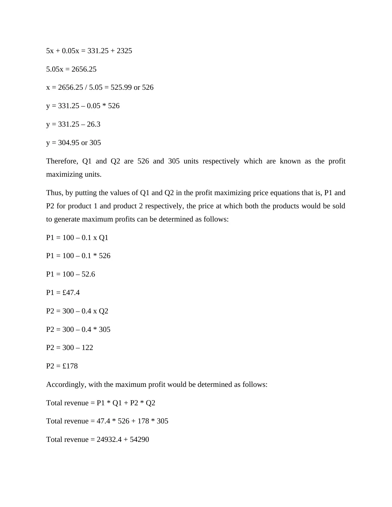
5x + 0.05x = 331.25 + 2325
5.05x = 2656.25
x = 2656.25 / 5.05 = 525.99 or 526
y = 331.25 – 0.05 * 526
y = 331.25 – 26.3
y = 304.95 or 305
Therefore, Q1 and Q2 are 526 and 305 units respectively which are known as the profit
maximizing units.
Thus, by putting the values of Q1 and Q2 in the profit maximizing price equations that is, P1 and
P2 for product 1 and product 2 respectively, the price at which both the products would be sold
to generate maximum profits can be determined as follows:
P1 = 100 – 0.1 x Q1
P1 = 100 – 0.1 * 526
P1 = 100 – 52.6
P1 = £47.4
P2 = 300 – 0.4 x Q2
P2 = 300 – 0.4 * 305
P2 = 300 – 122
P2 = £178
Accordingly, with the maximum profit would be determined as follows:
Total revenue = P1 * Q1 + P2 * Q2
Total revenue = 47.4 * 526 + 178 * 305
Total revenue = 24932.4 + 54290

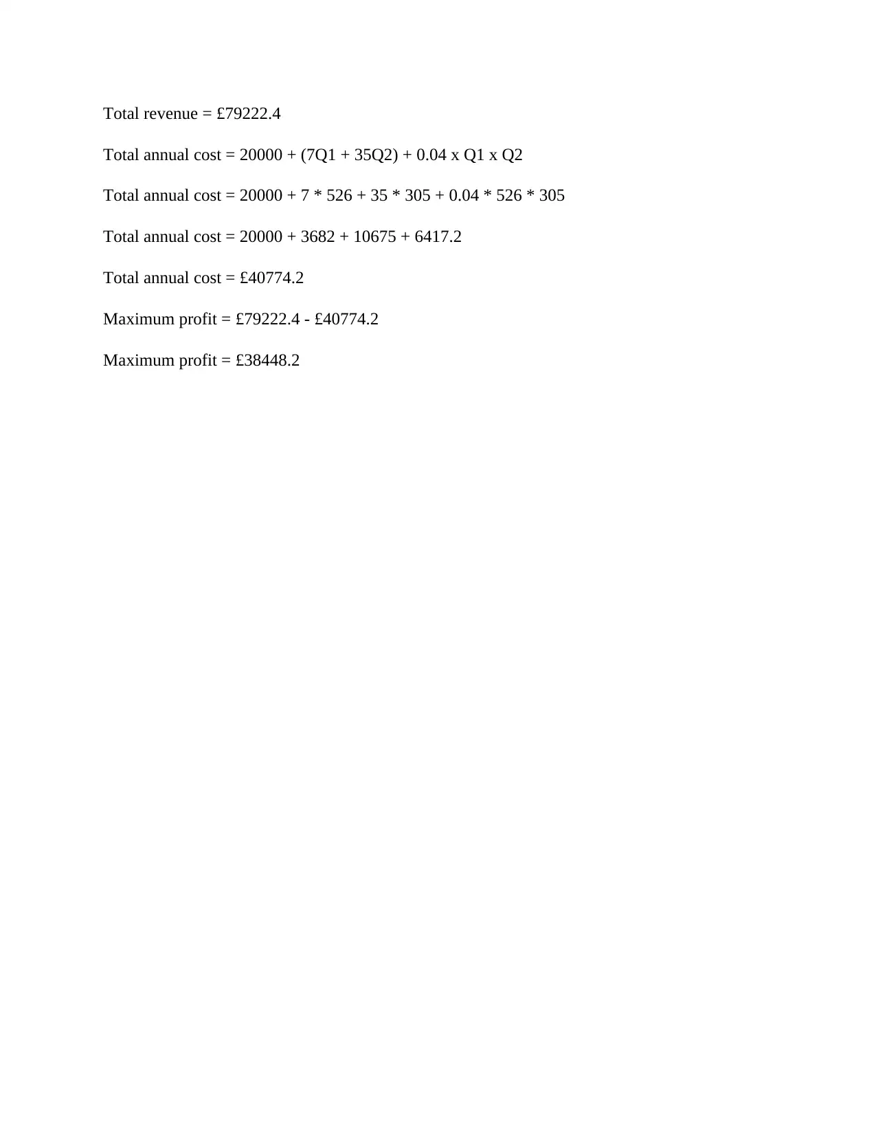
Total revenue = £79222.4
Total annual cost = 20000 + (7Q1 + 35Q2) + 0.04 x Q1 x Q2
Total annual cost = 20000 + 7 * 526 + 35 * 305 + 0.04 * 526 * 305
Total annual cost = 20000 + 3682 + 10675 + 6417.2
Total annual cost = £40774.2
Maximum profit = £79222.4 - £40774.2
Maximum profit = £38448.2

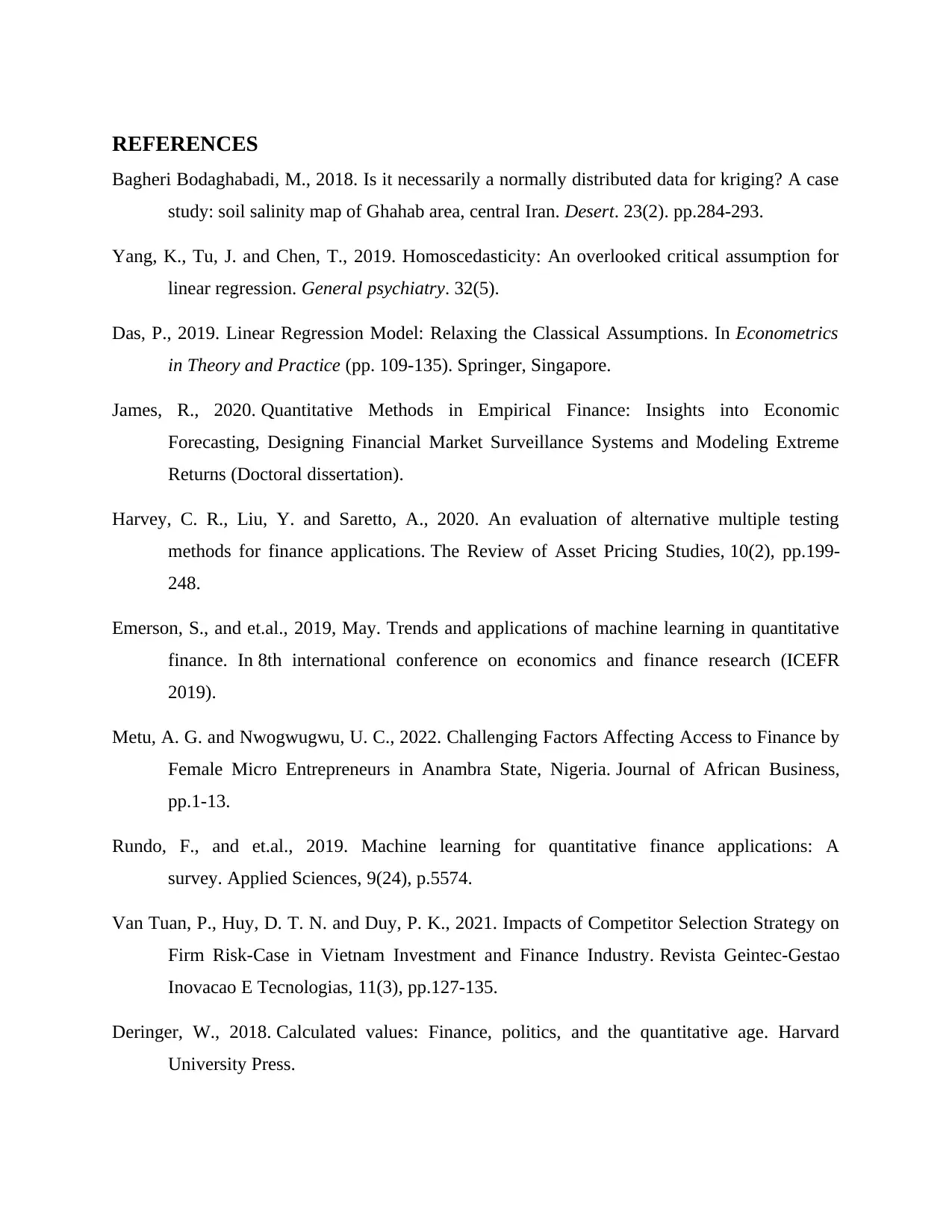
REFERENCES
Bagheri Bodaghabadi, M., 2018. Is it necessarily a normally distributed data for kriging? A case
study: soil salinity map of Ghahab area, central Iran. Desert. 23(2). pp.284-293.
Yang, K., Tu, J. and Chen, T., 2019. Homoscedasticity: An overlooked critical assumption for
linear regression. General psychiatry. 32(5).
Das, P., 2019. Linear Regression Model: Relaxing the Classical Assumptions. In Econometrics
in Theory and Practice (pp. 109-135). Springer, Singapore.
James, R., 2020. Quantitative Methods in Empirical Finance: Insights into Economic
Forecasting, Designing Financial Market Surveillance Systems and Modeling Extreme
Returns (Doctoral dissertation).
Harvey, C. R., Liu, Y. and Saretto, A., 2020. An evaluation of alternative multiple testing
methods for finance applications. The Review of Asset Pricing Studies, 10(2), pp.199-
248.
Emerson, S., and et.al., 2019, May. Trends and applications of machine learning in quantitative
finance. In 8th international conference on economics and finance research (ICEFR
2019).
Metu, A. G. and Nwogwugwu, U. C., 2022. Challenging Factors Affecting Access to Finance by
Female Micro Entrepreneurs in Anambra State, Nigeria. Journal of African Business,
pp.1-13.
Rundo, F., and et.al., 2019. Machine learning for quantitative finance applications: A
survey. Applied Sciences, 9(24), p.5574.
Van Tuan, P., Huy, D. T. N. and Duy, P. K., 2021. Impacts of Competitor Selection Strategy on
Firm Risk-Case in Vietnam Investment and Finance Industry. Revista Geintec-Gestao
Inovacao E Tecnologias, 11(3), pp.127-135.
Deringer, W., 2018. Calculated values: Finance, politics, and the quantitative age. Harvard
University Press.