Identifying Primary and Secondary Sources

This document discusses the difference between primary and secondary sources and provides examples for each. It also explains the appropriate data collection methods for different situations and the most suitable sampling methods. Additionally, it defines different types of data and provides examples. The document concludes with discussions on correlation, scatter diagrams, and statistical analysis.

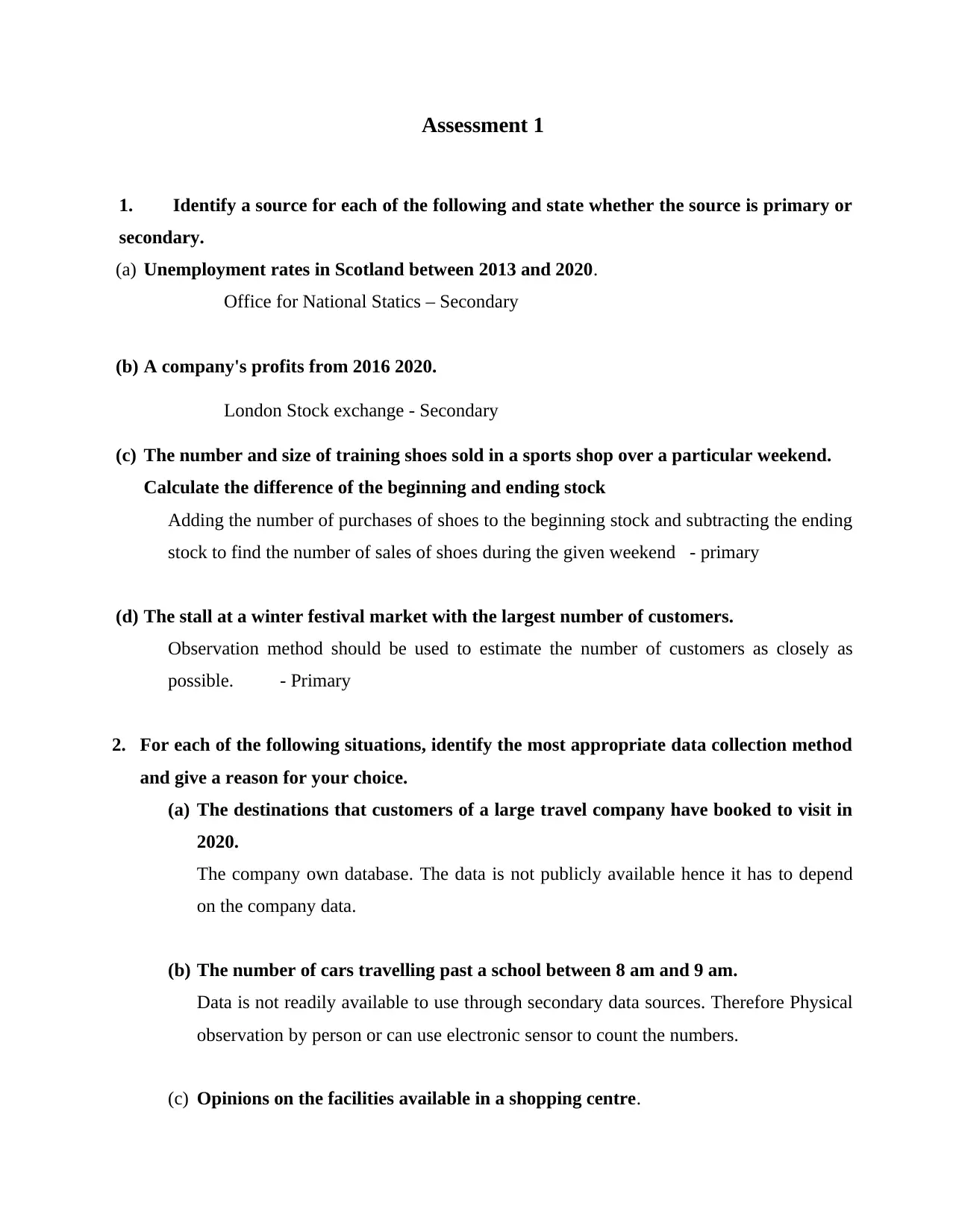
Assessment 1
1. Identify a source for each of the following and state whether the source is primary or
secondary.
(a) Unemployment rates in Scotland between 2013 and 2020.
Office for National Statics – Secondary
(b) A company's profits from 2016 2020.
London Stock exchange - Secondary
(c) The number and size of training shoes sold in a sports shop over a particular weekend.
Calculate the difference of the beginning and ending stock
Adding the number of purchases of shoes to the beginning stock and subtracting the ending
stock to find the number of sales of shoes during the given weekend - primary
(d) The stall at a winter festival market with the largest number of customers.
Observation method should be used to estimate the number of customers as closely as
possible. - Primary
2. For each of the following situations, identify the most appropriate data collection method
and give a reason for your choice.
(a) The destinations that customers of a large travel company have booked to visit in
2020.
The company own database. The data is not publicly available hence it has to depend
on the company data.
(b) The number of cars travelling past a school between 8 am and 9 am.
Data is not readily available to use through secondary data sources. Therefore Physical
observation by person or can use electronic sensor to count the numbers.
(c) Opinions on the facilities available in a shopping centre.

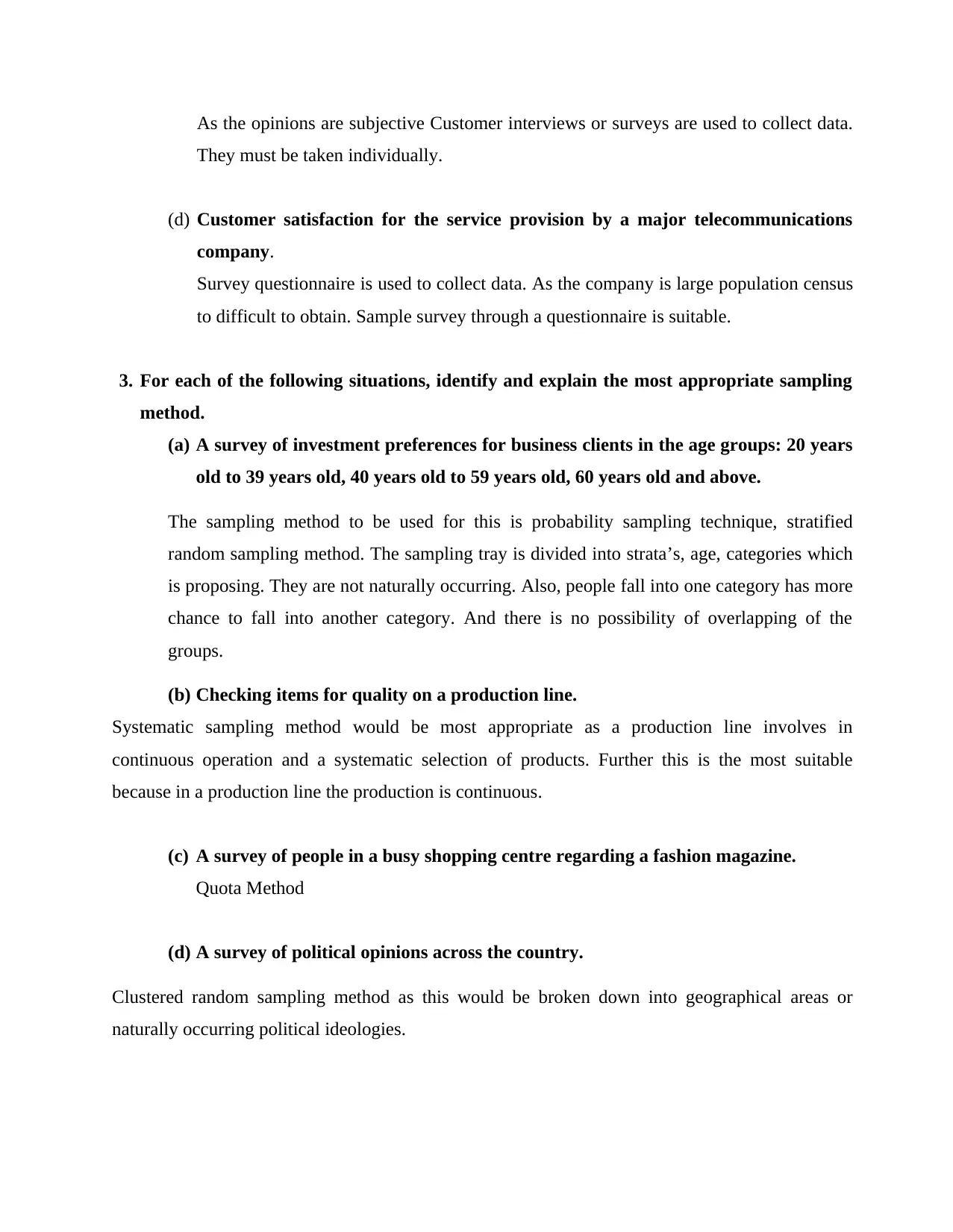
As the opinions are subjective Customer interviews or surveys are used to collect data.
They must be taken individually.
(d) Customer satisfaction for the service provision by a major telecommunications
company.
Survey questionnaire is used to collect data. As the company is large population census
to difficult to obtain. Sample survey through a questionnaire is suitable.
3. For each of the following situations, identify and explain the most appropriate sampling
method.
(a) A survey of investment preferences for business clients in the age groups: 20 years
old to 39 years old, 40 years old to 59 years old, 60 years old and above.
The sampling method to be used for this is probability sampling technique, stratified
random sampling method. The sampling tray is divided into strata’s, age, categories which
is proposing. They are not naturally occurring. Also, people fall into one category has more
chance to fall into another category. And there is no possibility of overlapping of the
groups.
(b) Checking items for quality on a production line.
Systematic sampling method would be most appropriate as a production line involves in
continuous operation and a systematic selection of products. Further this is the most suitable
because in a production line the production is continuous.
(c) A survey of people in a busy shopping centre regarding a fashion magazine.
Quota Method
(d) A survey of political opinions across the country.
Clustered random sampling method as this would be broken down into geographical areas or
naturally occurring political ideologies.

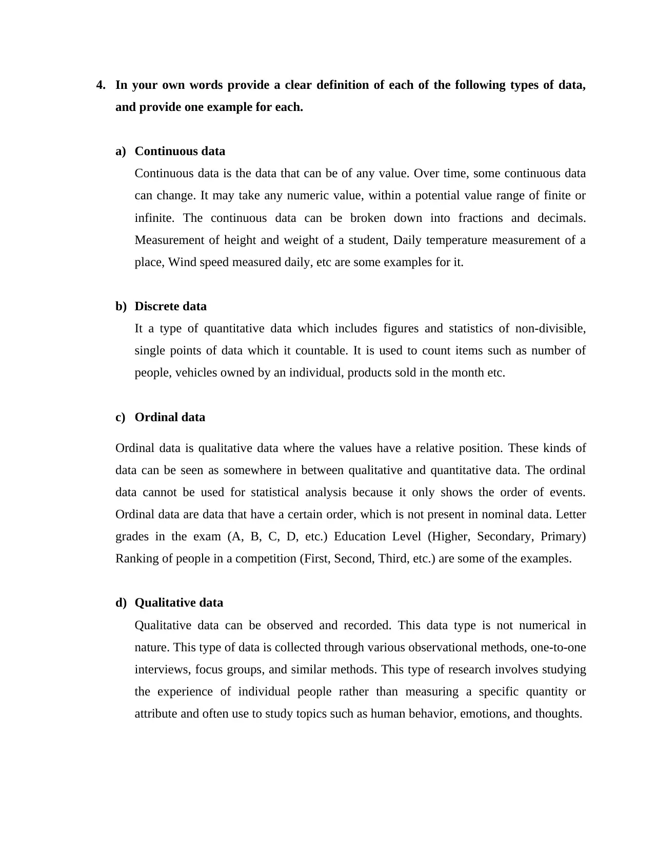
4. In your own words provide a clear definition of each of the following types of data,
and provide one example for each.
a) Continuous data
Continuous data is the data that can be of any value. Over time, some continuous data
can change. It may take any numeric value, within a potential value range of finite or
infinite. The continuous data can be broken down into fractions and decimals.
Measurement of height and weight of a student, Daily temperature measurement of a
place, Wind speed measured daily, etc are some examples for it.
b) Discrete data
It a type of quantitative data which includes figures and statistics of non-divisible,
single points of data which it countable. It is used to count items such as number of
people, vehicles owned by an individual, products sold in the month etc.
c) Ordinal data
Ordinal data is qualitative data where the values have a relative position. These kinds of
data can be seen as somewhere in between qualitative and quantitative data. The ordinal
data cannot be used for statistical analysis because it only shows the order of events.
Ordinal data are data that have a certain order, which is not present in nominal data. Letter
grades in the exam (A, B, C, D, etc.) Education Level (Higher, Secondary, Primary)
Ranking of people in a competition (First, Second, Third, etc.) are some of the examples.
d) Qualitative data
Qualitative data can be observed and recorded. This data type is not numerical in
nature. This type of data is collected through various observational methods, one-to-one
interviews, focus groups, and similar methods. This type of research involves studying
the experience of individual people rather than measuring a specific quantity or
attribute and often use to study topics such as human behavior, emotions, and thoughts.

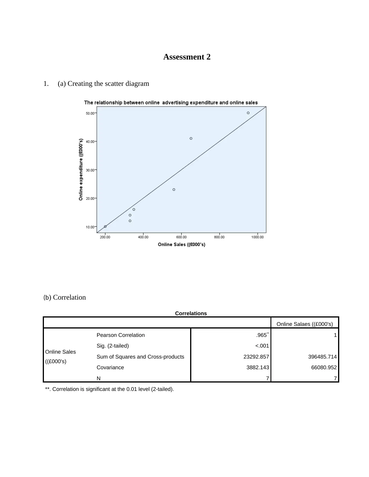
Assessment 2
1. (a) Creating the scatter diagram
(b) Correlation
Correlations
Online Salaes ((£000's)
Online Sales
((£000's)
Pearson Correlation .965** 1
Sig. (2-tailed) <.001
Sum of Squares and Cross-products 23292.857 396485.714
Covariance 3882.143 66080.952
N 7 7
**. Correlation is significant at the 0.01 level (2-tailed).

(c )
Coefficientsa
Model Unstandardized
Coefficients
Standardized
Coefficients t Sig. 95.0% Confidence
Interval for B
Correlations Collinearity
Statistics
B Std.
Error
Beta Lower
Bound
Upper
Bound
Zero-
order
Partial Part Tolerance VIF
1
(Constant) 105.518 53.525 1.971 .106 -32.073 243.109
Online
expenditure
((£000's)
15.852 1.926 .965 8.230 .000 10.901 20.803 .965 .965 .965 1.000 1.000
a. Dependent Variable: Online Salaes ((£000's)
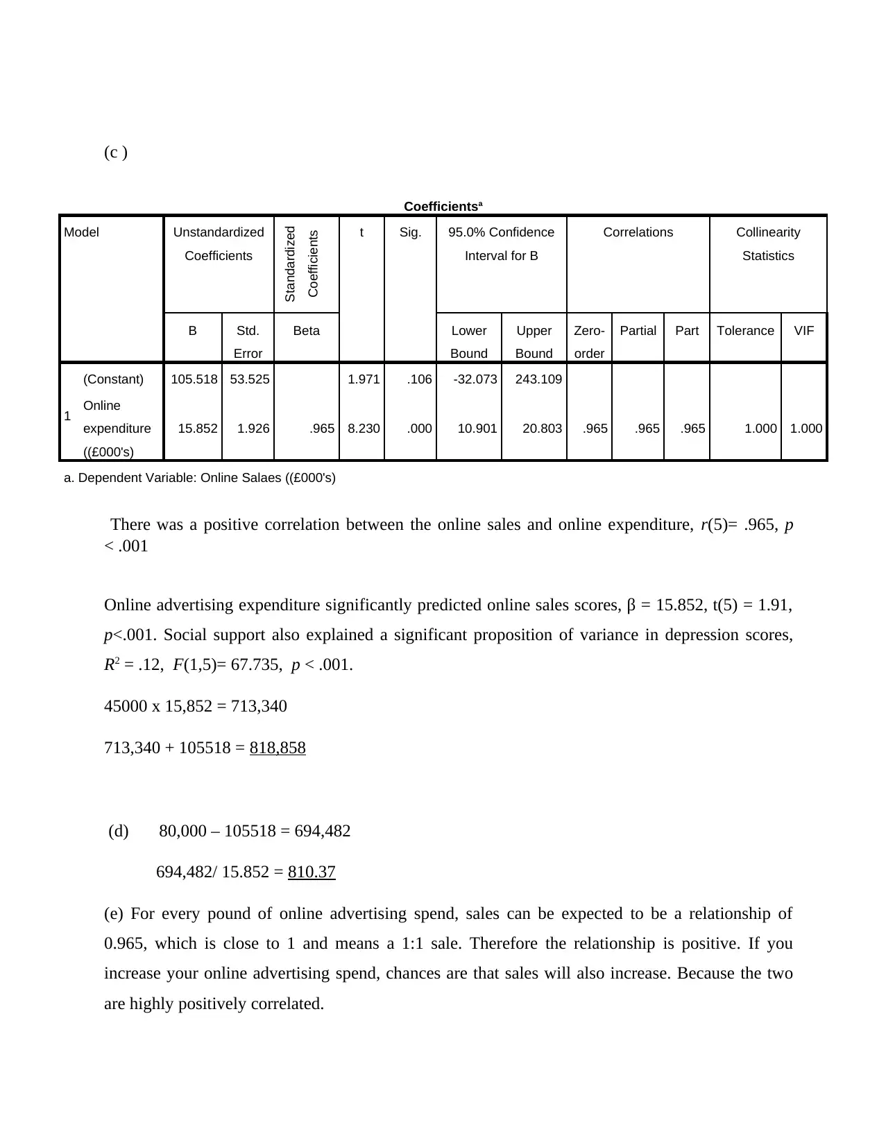
There was a positive correlation between the online sales and online expenditure, r(5)= .965, p
< .001
Online advertising expenditure significantly predicted online sales scores, β = 15.852, t(5) = 1.91,
p<.001. Social support also explained a significant proposition of variance in depression scores,
R2 = .12, F(1,5)= 67.735, p < .001.
45000 x 15,852 = 713,340
713,340 + 105518 = 818,858
(d) 80,000 – 105518 = 694,482
694,482/ 15.852 = 810.37
(e) For every pound of online advertising spend, sales can be expected to be a relationship of
0.965, which is close to 1 and means a 1:1 sale. Therefore the relationship is positive. If you
increase your online advertising spend, chances are that sales will also increase. Because the two
are highly positively correlated.

2. (a)
38%
26%
12%
11%
14%
Aberdeen
Excellent Good Fair Poor Very poor
Aberdeen Glasgow
Excellent 28 53
Good 19 64
Fair 9 60
Poor 8 12
Very poor 10 7

27%
33%
31%
6% 4%
Glasgow
Excellent Good Fair Poor Very poor
Excellent Good Fair Poor Very poor
0
10
20
30
40
50
60
70
Customer Service Rating
Aberdeen Glasgow
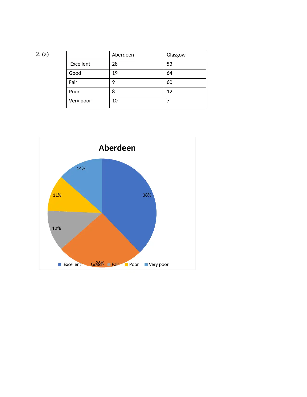
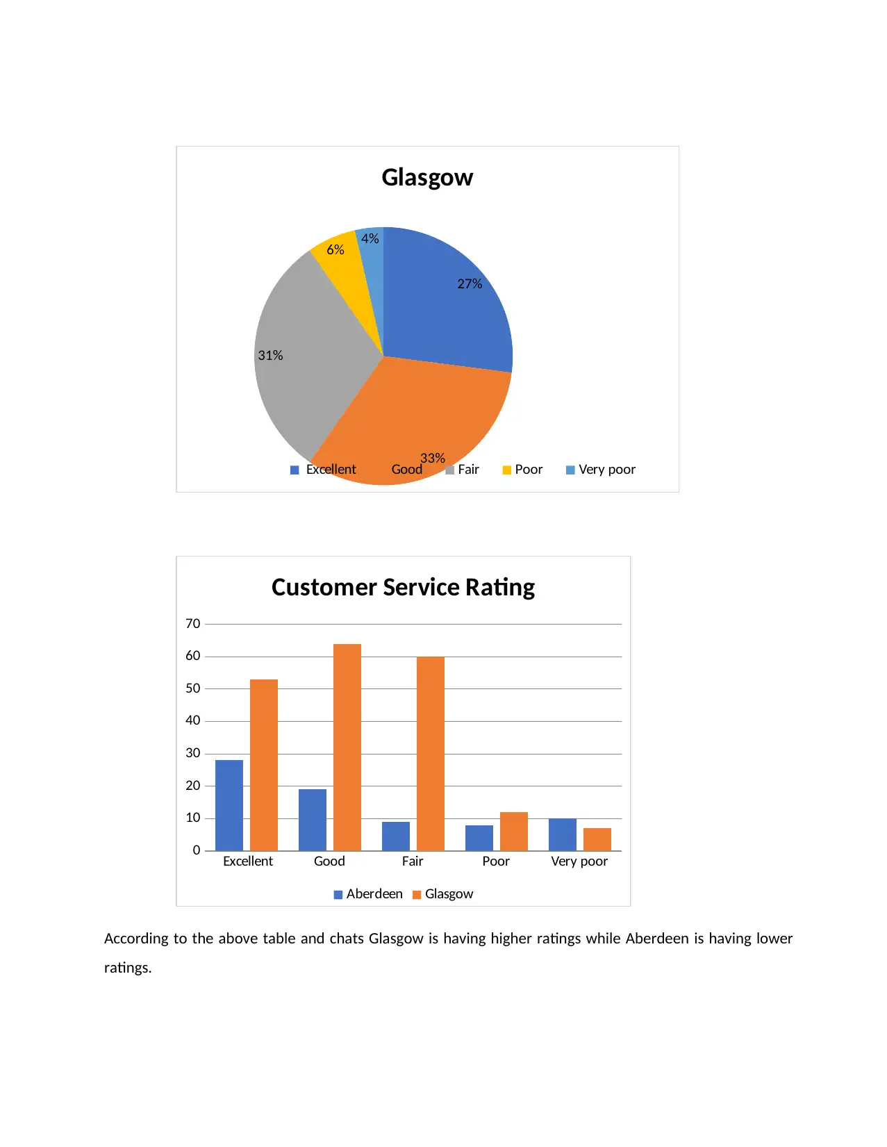
According to the above table and chats Glasgow is having higher ratings while Aberdeen is having lower
ratings.

3.
Tea Coffee Hot chocolate Water
0
20
40
60
80
100
120
140
160
Number of drinks sold
Morning Afternoon Evening
3. Drink Morning Afternoon Evening
Tea 80 136 26
Coffee 146 102 58
Hot chocolate 26 16 32
Water 32 74 94

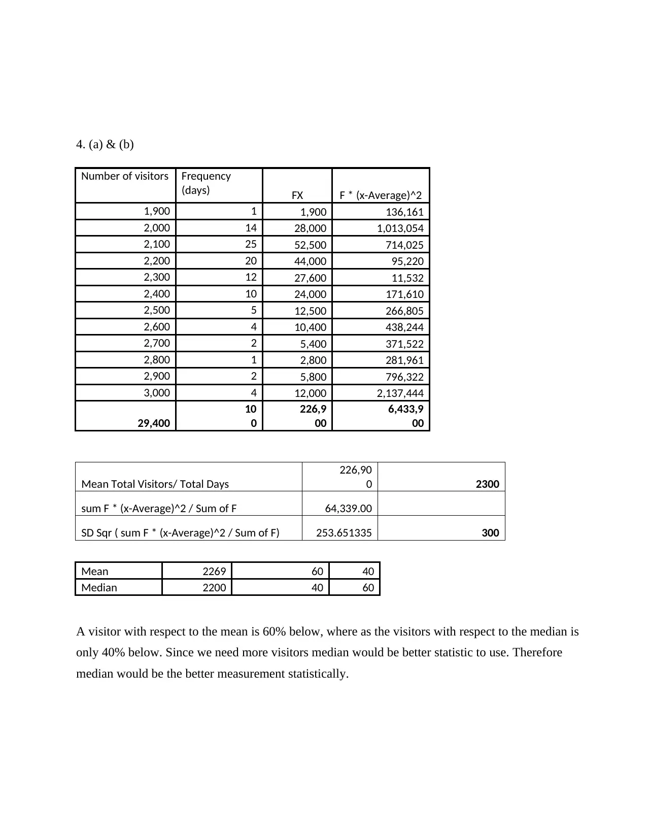
4. (a) & (b)
Number of visitors Frequency
(days) FX F * (x-Average)^2
1,900 1 1,900 136,161
2,000 14 28,000 1,013,054
2,100 25 52,500 714,025
2,200 20 44,000 95,220
2,300 12 27,600 11,532
2,400 10 24,000 171,610
2,500 5 12,500 266,805
2,600 4 10,400 438,244
2,700 2 5,400 371,522
2,800 1 2,800 281,961
2,900 2 5,800 796,322
3,000 4 12,000 2,137,444
29,400
10
0
226,9
00
6,433,9
00
Mean Total Visitors/ Total Days
226,90
0 2300
sum F * (x-Average)^2 / Sum of F 64,339.00
SD Sqr ( sum F * (x-Average)^2 / Sum of F) 253.651335 300
Mean 2269 60 40
Median 2200 40 60
A visitor with respect to the mean is 60% below, where as the visitors with respect to the median is
only 40% below. Since we need more visitors median would be better statistic to use. Therefore
median would be the better measurement statistically.

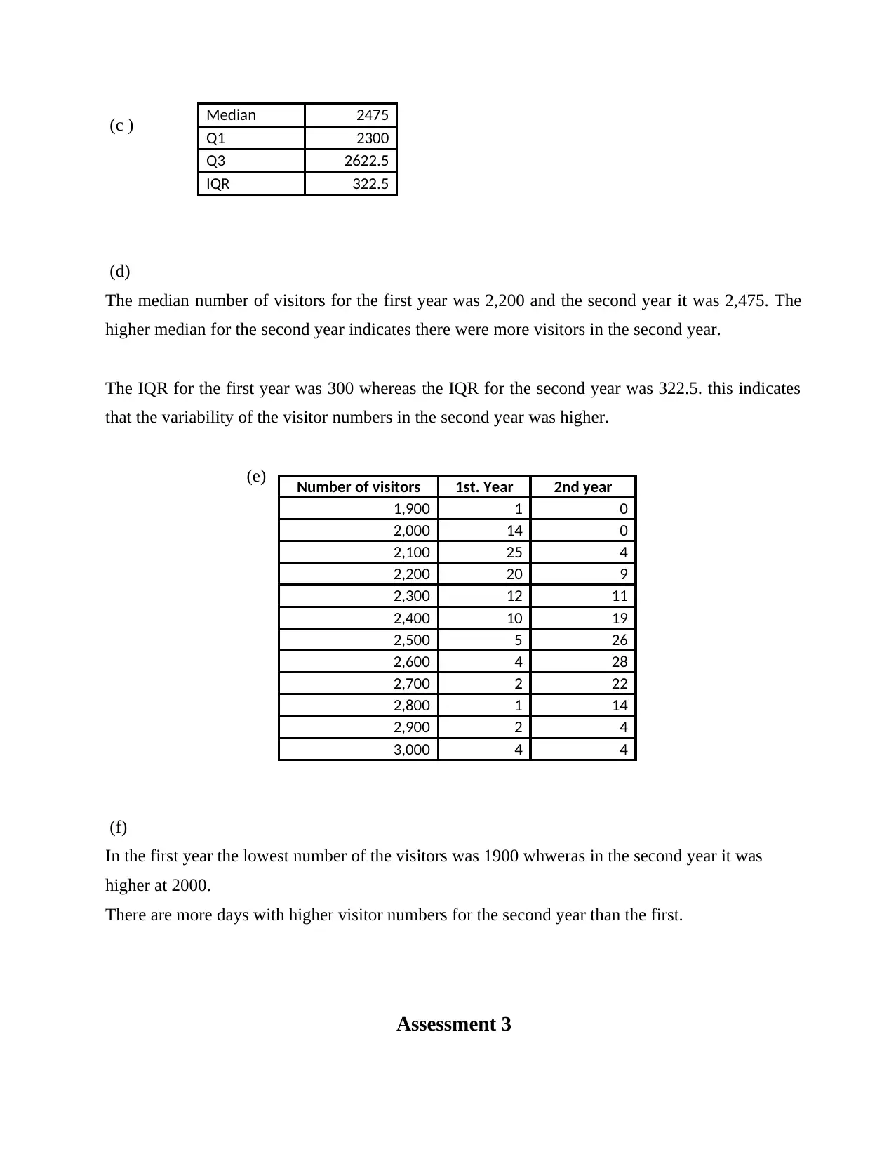
(c )
(d)
The median number of visitors for the first year was 2,200 and the second year it was 2,475. The
higher median for the second year indicates there were more visitors in the second year.
The IQR for the first year was 300 whereas the IQR for the second year was 322.5. this indicates
that the variability of the visitor numbers in the second year was higher.
(e)
(f)
In the first year the lowest number of the visitors was 1900 whweras in the second year it was
higher at 2000.
There are more days with higher visitor numbers for the second year than the first.
Assessment 3
Median 2475
Q1 2300
Q3 2622.5
IQR 322.5
Number of visitors 1st. Year 2nd year
1,900 1 0
2,000 14 0
2,100 25 4
2,200 20 9
2,300 12 11
2,400 10 19
2,500 5 26
2,600 4 28
2,700 2 22
2,800 1 14
2,900 2 4
3,000 4 4

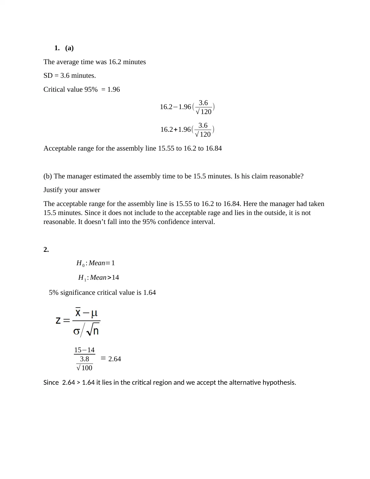
1. (a)
The average time was 16.2 minutes
SD = 3.6 minutes.
Critical value 95% = 1.96
16.2−1.96 ( 3.6
√ 120 )
16.2+1.96( 3.6
√ 120 )
Acceptable range for the assembly line 15.55 to 16.2 to 16.84
(b) The manager estimated the assembly time to be 15.5 minutes. Is his claim reasonable?
Justify your answer
The acceptable range for the assembly line is 15.55 to 16.2 to 16.84. Here the manager had taken
15.5 minutes. Since it does not include to the acceptable rage and lies in the outside, it is not
reasonable. It doesn’t fall into the 95% confidence interval.
2.
H0 : Mean=1
H1 : Mean >14
5% significance critical value is 1.64
15−14
3.8
√ 100
= 2.64
Since 2.64 > 1.64 it lies in the critical region and we accept the alternative hypothesis.

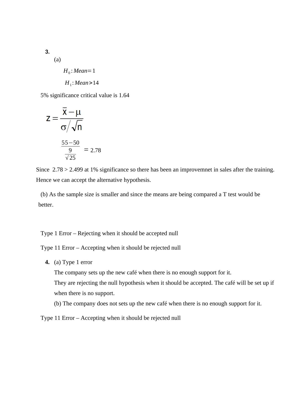
3.
(a)
H0 : Mean=1
H1 : Mean >14
5% significance critical value is 1.64
55−50
9
√ 25
= 2.78
Since 2.78 > 2.499 at 1% significance so there has been an improvemnet in sales after the training.
Hence we can accept the alternative hypothesis.
(b) As the sample size is smaller and since the means are being compared a T test would be
better.
Type 1 Error – Rejecting when it should be accepted null
Type 11 Error – Accepting when it should be rejected null
4. (a) Type 1 error
The company sets up the new café when there is no enough support for it.
They are rejecting the null hypothesis when it should be accepted. The café will be set up if
when there is no support.
(b) The company does not sets up the new café when there is no enough support for it.
Type 11 Error – Accepting when it should be rejected null