Investment Portfolio Risk-Return Analysis
VerifiedAdded on 2020/07/22
|21
|2708
|219
AI Summary
This assignment involves evaluating three given investment portfolios using various financial analysis tools such as Sharpe Ratio, Security Market Line (SML), Capital Market Line (CML), and regression analysis. The primary goal is to identify the best portfolio option available to an investor in terms of risk-adjusted return, while also understanding the relationship between these portfolios and their corresponding Sharpe ratios.
Contribute Materials
Your contribution can guide someone’s learning journey. Share your
documents today.

BUSINESS FINANCE
Secure Best Marks with AI Grader
Need help grading? Try our AI Grader for instant feedback on your assignments.


EXECUTIVE SUMMARY
Investment is made by all sort of people in terms of income level but making prudent decisions
is very difficult task. In order to take perfect decision some tools and techniques need to be used.
In the present research study index return and firms returns are analyzed by using tools like
mean , standard deviation and beta. It is observed that security markert line is the one of the
important approach that help one in making correct decisions. By comparing requred rate of
return with market return it is identified whether investment must be made in specific security or
not. Beta is another tool that must be widely used in order to meausre risk and to make
decisions. Thus, investors must not rely on single approach as they must use multiple methods to
take investment decisions.
TABLE OF CONTENTS
INTRODUCTION...........................................................................................................................1
REQUIRED.....................................................................................................................................1
(1)Monthly return series of stocks and index..............................................................................1
(2)Portolio construction...............................................................................................................1
(3) Mean return and standard deviation of stock, index and portfolio........................................2
(4) Regression analysis................................................................................................................3
(3) Beta estimates of portfolio...................................................................................................12
5 Combination line chart...........................................................................................................24
ANALYSIS....................................................................................................................................24
(1)Performance of market and six stocks..................................................................................24
(2) Comparison of portfolios.....................................................................................................25
(3) Relationship between sharpe ratio portfolio 3,2 and chart ploted in 5th point.....................25
(4) SML and CML.....................................................................................................................25
5 Discussion on calculations......................................................................................................26
CONCLUSION..............................................................................................................................26
REFERENCES..............................................................................................................................27
Figure 1Mean and standard deviation chart...................................................................................13
Figure 2Mean and beta chart.........................................................................................................13
Figure 3Mean and standard deviation chart...................................................................................14
Figure 4Mean and beta chart.........................................................................................................14
Figure 5Mean and standard deviation chart...................................................................................15
Figure 6Mean and beta chart.........................................................................................................15
Figure 7Mean and standard deviation chart...................................................................................16
Figure 8Mean and beta chart.........................................................................................................16
Figure 9Mean and standard deviation chart...................................................................................17
Secure Best Marks with AI Grader
Need help grading? Try our AI Grader for instant feedback on your assignments.
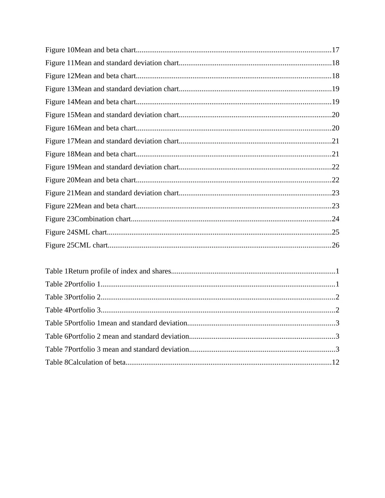
Figure 10Mean and beta chart.......................................................................................................17
Figure 11Mean and standard deviation chart.................................................................................18
Figure 12Mean and beta chart.......................................................................................................18
Figure 13Mean and standard deviation chart.................................................................................19
Figure 14Mean and beta chart.......................................................................................................19
Figure 15Mean and standard deviation chart.................................................................................20
Figure 16Mean and beta chart.......................................................................................................20
Figure 17Mean and standard deviation chart.................................................................................21
Figure 18Mean and beta chart.......................................................................................................21
Figure 19Mean and standard deviation chart.................................................................................22
Figure 20Mean and beta chart.......................................................................................................22
Figure 21Mean and standard deviation chart.................................................................................23
Figure 22Mean and beta chart.......................................................................................................23
Figure 23Combination chart..........................................................................................................24
Figure 24SML chart.......................................................................................................................25
Figure 25CML chart......................................................................................................................26
Table 1Return profile of index and shares.......................................................................................1
Table 2Portfolio 1............................................................................................................................1
Table 3Portfolio 2............................................................................................................................2
Table 4Portfolio 3............................................................................................................................2
Table 5Portfolio 1mean and standard deviation..............................................................................3
Table 6Portfolio 2 mean and standard deviation.............................................................................3
Table 7Portfolio 3 mean and standard deviation.............................................................................3
Table 8Calculation of beta.............................................................................................................12
INTRODUCTION
Investment is one of the important area that is related to every human being whether it
comes in upper or middle classs. There are number of tools and techniques that need to be used
in order to make prudent decisions. In current report, portfolios are created and varied tools are
used like beta and standard deviation, CML and SML for evaluating stocks and identifying
varied facts. In second part of report all results are discussed and in this way entire research work
is done.
REQUIRED
Introduction to firms ANZ: ANZ is also known by name Australia and New Zealand Banking group as it is one
of the largest bank of Australia in terms of market capitalization. Currently, firm is
offering number of products to its customers whether they are retail or HNI. Firm have its
own future plans and have good growth prospects. BHP: BHP is one of well known firm that is operating in mines, metals and petroleum
products. It is Australia largest mining company in terms of turnover. Presently, firm is
operating its business in number of nations of world and have good growth rate in
business. CSL: It is a company operating in biotechnology field. There are number of areas in this
field and CSL is operating streams from where good amount of cash flow can be
received. Firm product portfolio is wide and also provide good quality of services to
customers. FMG: It is largest iron ore company and is considered as one of the largest iron mineral
marker in the world. FMG is considered as greater in size in comparison to rivals Rio
Tinto and BHP. FMG have USP which make it different from rivals. WOW: It is a retail firm that is operating in both Australia and New Zelanad. Firm is
consistently opening new branches in foreign nations and is earning good amount of
revenue in the business. Thus, it can be said that with improvement in global economy
good profit will be earned by the firm.
(1)Monthly return series of stocks and index
Table 1Return profile of index and shares
Compan Return
1 | P a g e
y
ANZ -0.0147
BHP
-
0.63789
CSL
1.83907
1
FMG
-
0.60218
TLS
0.89007
1
XAOA 0.30238
(2)Portolio construction
Table 2Portfolio 1
Portfolio 1
Weig
ht Value
ANZ 0.5 -0.0147
-
0.00735
BHP 0.5
-
0.63789
-
0.31894
CSL 0.5
1.83907
1
0.91953
5
FMG 0.5
-
0.60218
-
0.30109
TLS 0.5 0.89
0.44503
5
WOW 0.5
-
0.17783
-
0.08891
Return
0.64827
2
2 | P a g e
Paraphrase This Document
Need a fresh take? Get an instant paraphrase of this document with our AI Paraphraser
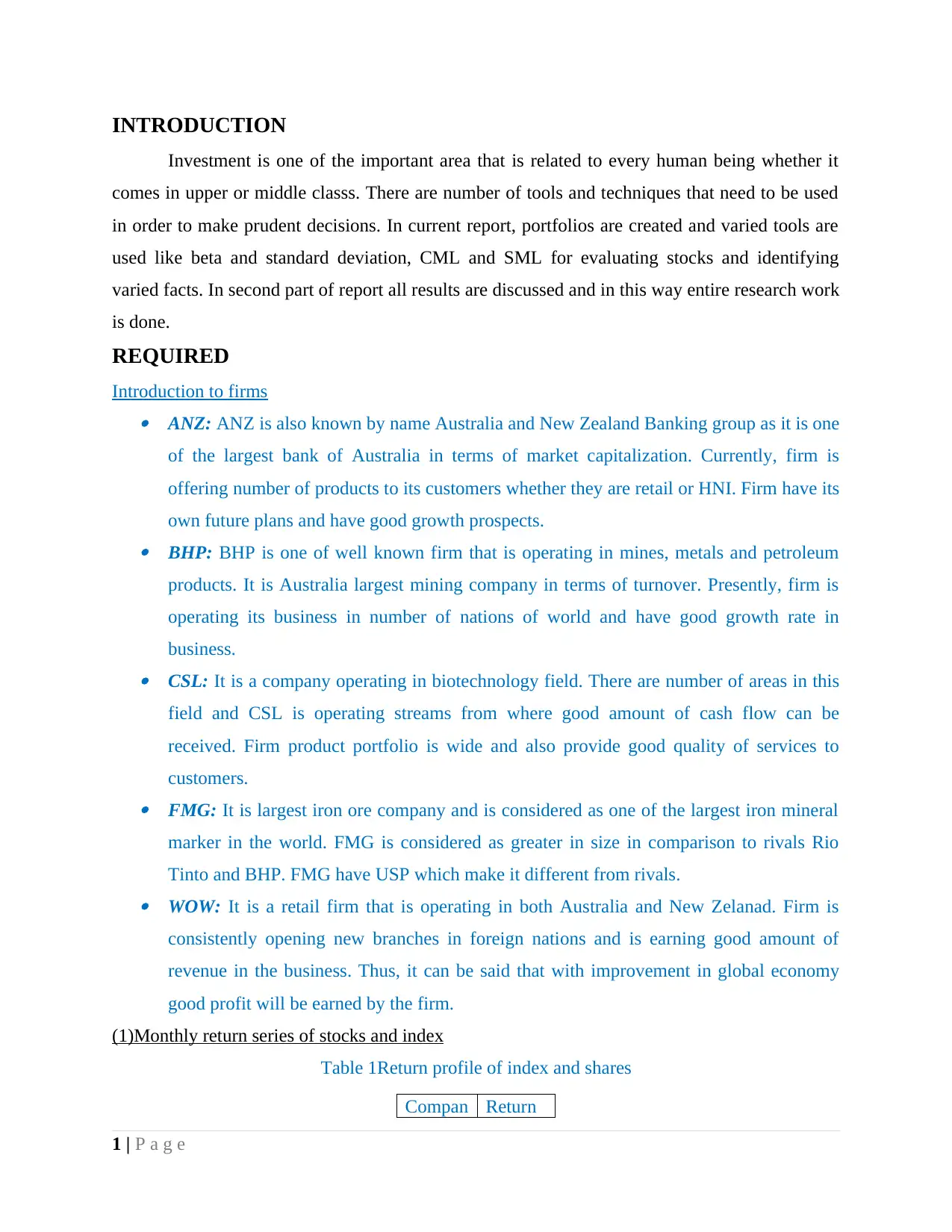
Mean STDEV
0
0.1
0.2
0.3
0.4
0.5
0.6
0.10804532988083
5
0.48454103502003
6
Chart Title
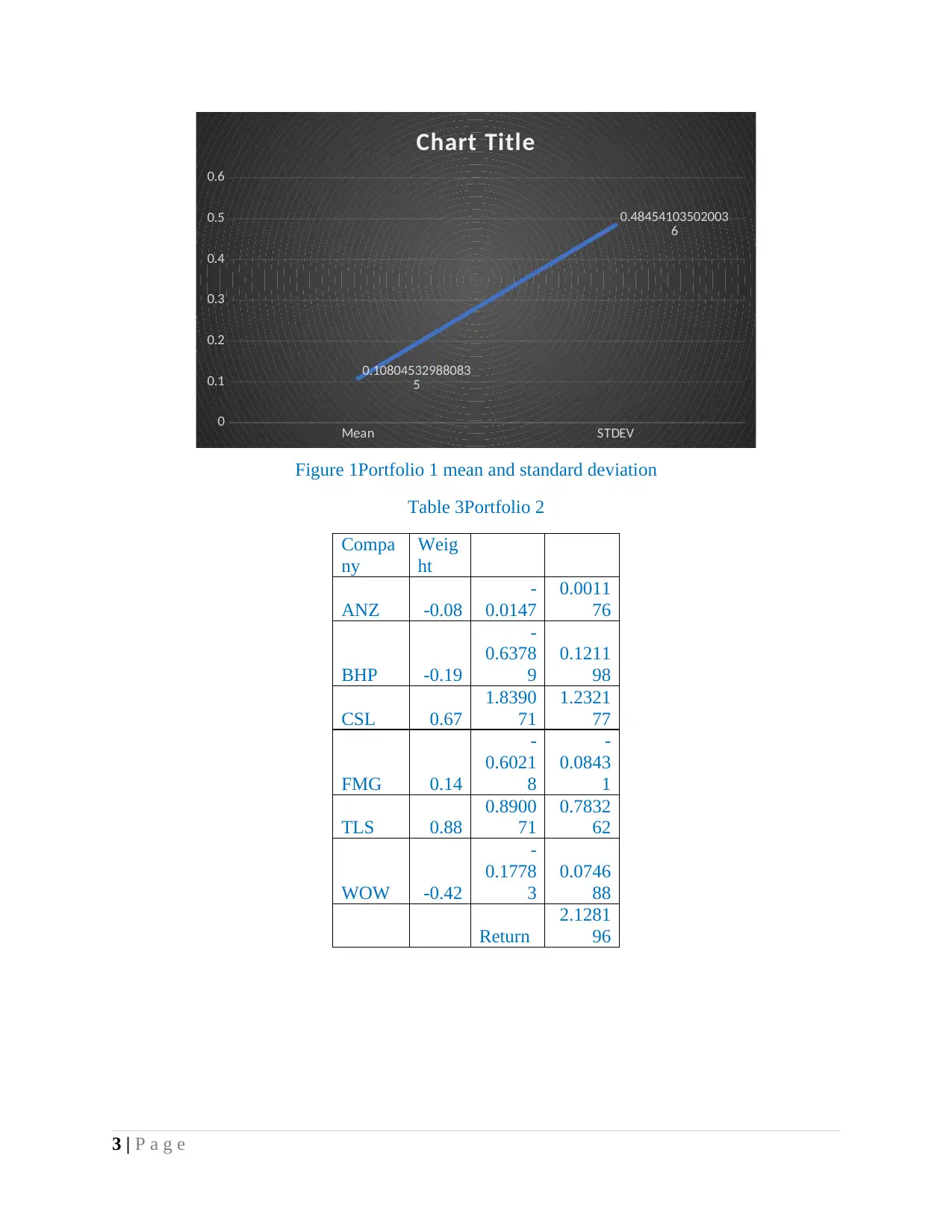
Figure 1Portfolio 1 mean and standard deviation
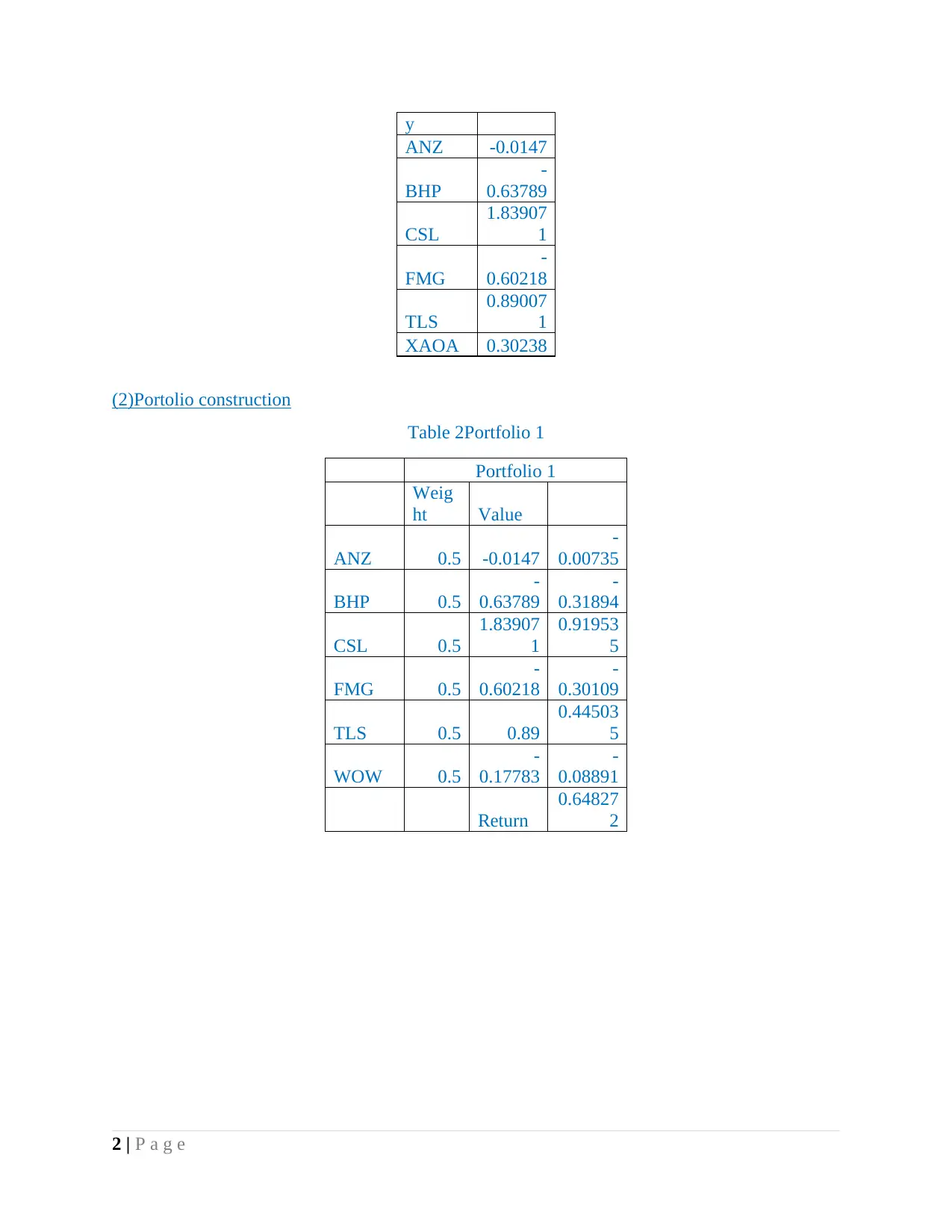
Table 3Portfolio 2
Compa
ny
Weig
ht
ANZ -0.08
-
0.0147
0.0011
76
BHP -0.19
-
0.6378
9
0.1211
98
CSL 0.67
1.8390
71
1.2321
77
FMG 0.14
-
0.6021
8
-
0.0843
1
TLS 0.88
0.8900
71
0.7832
62
WOW -0.42
-
0.1778
3
0.0746
88
Return
2.1281
96
3 | P a g e
0
0.1
0.2
0.3
0.4
0.5
0.6
0.10804532988083
5
0.48454103502003
6
Chart Title
Figure 1Portfolio 1 mean and standard deviation
Table 3Portfolio 2
Compa
ny
Weig
ht
ANZ -0.08
-
0.0147
0.0011
76
BHP -0.19
-
0.6378
9
0.1211
98
CSL 0.67
1.8390
71
1.2321
77
FMG 0.14
-
0.6021
8
-
0.0843
1
TLS 0.88
0.8900
71
0.7832
62
WOW -0.42
-
0.1778
3
0.0746
88
Return
2.1281
96
3 | P a g e
1 2
0
0.005
0.01
0.015
0.02
0.025
0.03
0.035
0.04
0.045
0.05
0.02504536555704
98
0.04502188619066
27
Chart Title
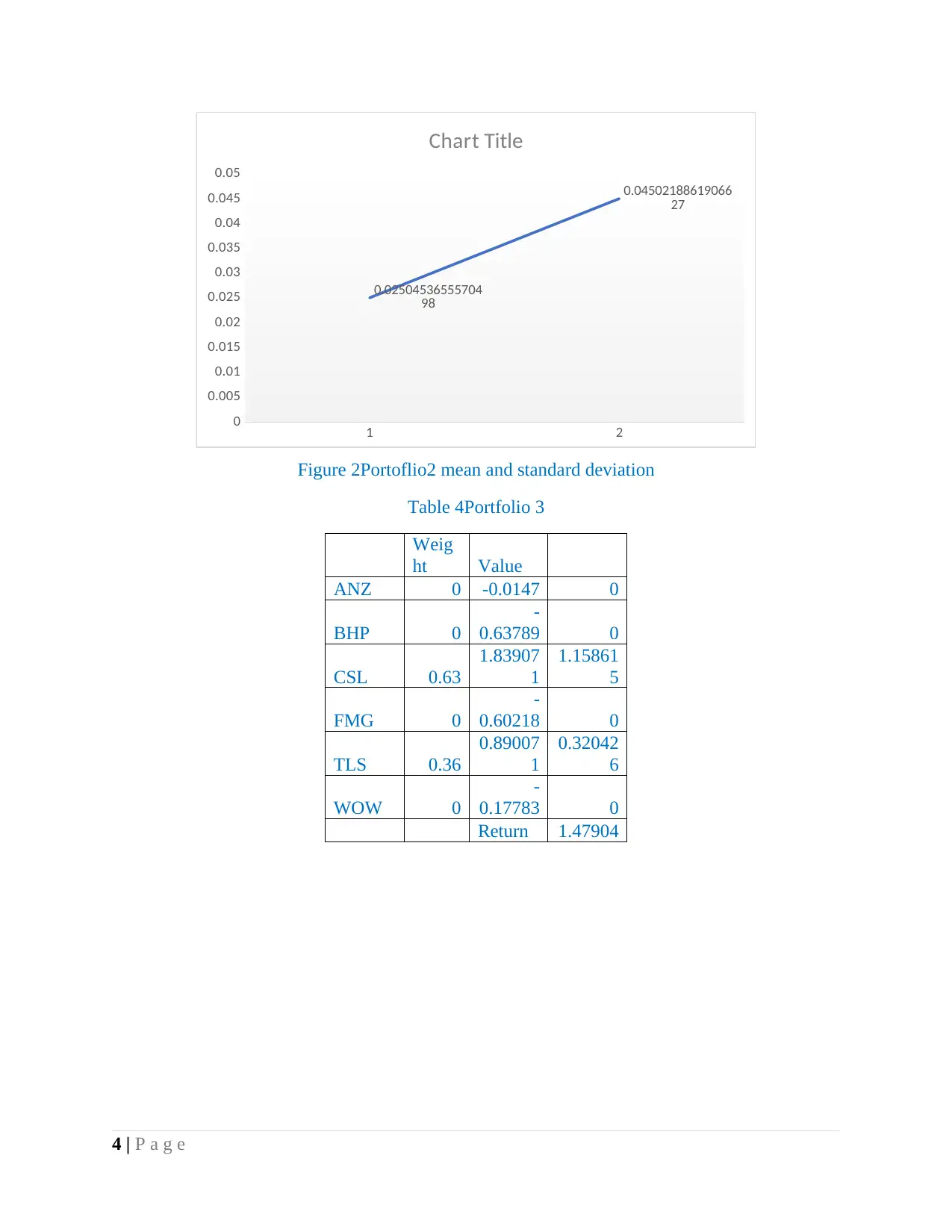
Figure 2Portoflio2 mean and standard deviation
Table 4Portfolio 3
Weig
ht Value
ANZ 0 -0.0147 0
BHP 0
-
0.63789 0
CSL 0.63
1.83907
1
1.15861
5
FMG 0
-
0.60218 0
TLS 0.36
0.89007
1
0.32042
6
WOW 0
-
0.17783 0
Return 1.47904
4 | P a g e
0
0.005
0.01
0.015
0.02
0.025
0.03
0.035
0.04
0.045
0.05
0.02504536555704
98
0.04502188619066
27
Chart Title
Figure 2Portoflio2 mean and standard deviation
Table 4Portfolio 3
Weig
ht Value
ANZ 0 -0.0147 0
BHP 0
-
0.63789 0
CSL 0.63
1.83907
1
1.15861
5
FMG 0
-
0.60218 0
TLS 0.36
0.89007
1
0.32042
6
WOW 0
-
0.17783 0
Return 1.47904
4 | P a g e
1 2
0.01608831666834
97
0.03953822865183
99
Chart Title
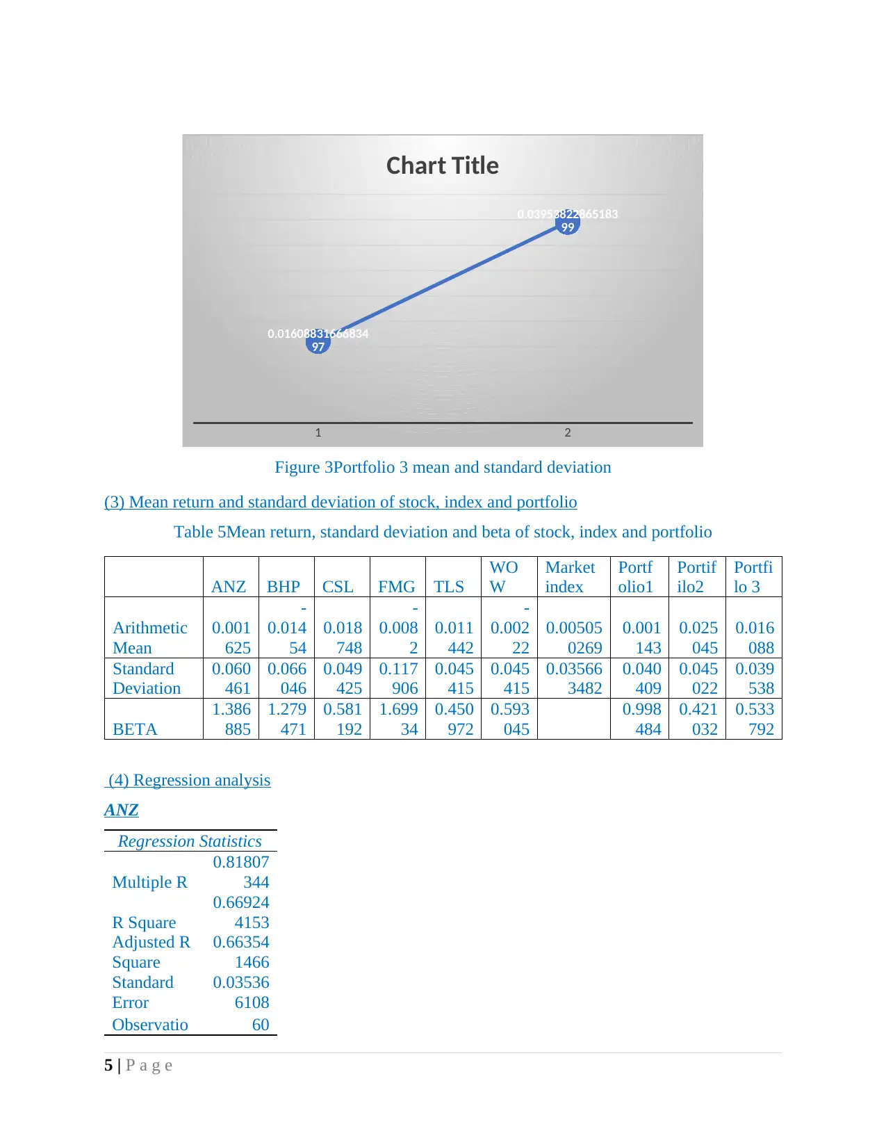
Figure 3Portfolio 3 mean and standard deviation
(3) Mean return and standard deviation of stock, index and portfolio
Table 5Mean return, standard deviation and beta of stock, index and portfolio
ANZ BHP CSL FMG TLS
WO
W
Market
index
Portf
olio1
Portif
ilo2
Portfi
lo 3
Arithmetic
Mean
0.001
625
-
0.014
54
0.018
748
-
0.008
2
0.011
442
-
0.002
22
0.00505
0269
0.001
143
0.025
045
0.016
088
Standard
Deviation
0.060
461
0.066
046
0.049
425
0.117
906
0.045
415
0.045
415
0.03566
3482
0.040
409
0.045
022
0.039
538
BETA
1.386
885
1.279
471
0.581
192
1.699
34
0.450
972
0.593
045
0.998
484
0.421
032
0.533
792
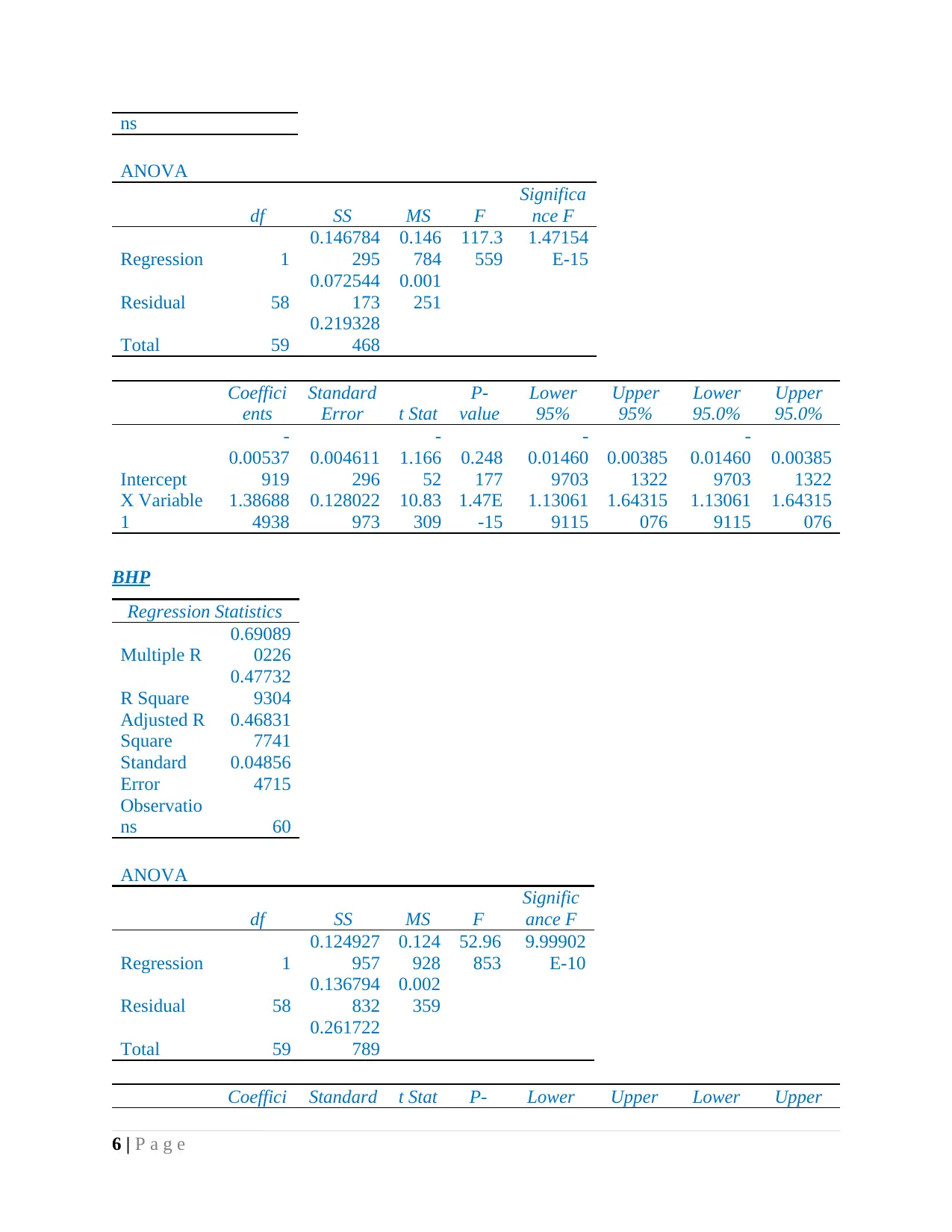
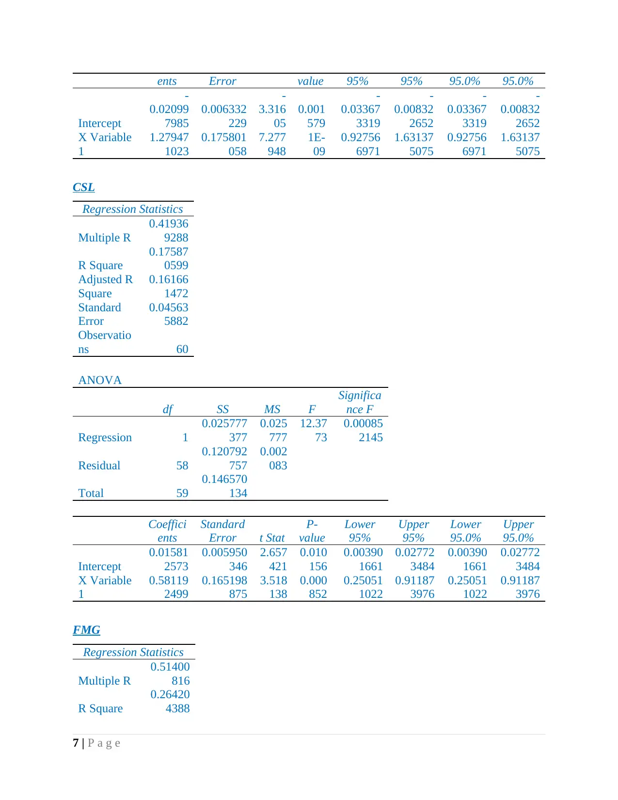
(4) Regression analysis
ANZ
Regression Statistics
Multiple R
0.81807
344
R Square
0.66924
4153
Adjusted R
Square
0.66354
1466
Standard
Error
0.03536
6108
Observatio 60
5 | P a g e
0.01608831666834
97
0.03953822865183
99
Chart Title
Figure 3Portfolio 3 mean and standard deviation
(3) Mean return and standard deviation of stock, index and portfolio
Table 5Mean return, standard deviation and beta of stock, index and portfolio
ANZ BHP CSL FMG TLS
WO
W
Market
index
Portf
olio1
Portif
ilo2
Portfi
lo 3
Arithmetic
Mean
0.001
625
-
0.014
54
0.018
748
-
0.008
2
0.011
442
-
0.002
22
0.00505
0269
0.001
143
0.025
045
0.016
088
Standard
Deviation
0.060
461
0.066
046
0.049
425
0.117
906
0.045
415
0.045
415
0.03566
3482
0.040
409
0.045
022
0.039
538
BETA
1.386
885
1.279
471
0.581
192
1.699
34
0.450
972
0.593
045
0.998
484
0.421
032
0.533
792
(4) Regression analysis
ANZ
Regression Statistics
Multiple R
0.81807
344
R Square
0.66924
4153
Adjusted R
Square
0.66354
1466
Standard
Error
0.03536
6108
Observatio 60
5 | P a g e
Secure Best Marks with AI Grader
Need help grading? Try our AI Grader for instant feedback on your assignments.
ns
ANOVA
df SS MS F
Significa
nce F
Regression 1
0.146784
295
0.146
784
117.3
559
1.47154
E-15
Residual 58
0.072544
173
0.001
251
Total 59
0.219328
468
Coeffici
ents
Standard
Error t Stat
P-
value
Lower
95%
Upper
95%
Lower
95.0%
Upper
95.0%
Intercept
-
0.00537
919
0.004611
296
-
1.166
52
0.248
177
-
0.01460
9703
0.00385
1322
-
0.01460
9703
0.00385
1322
X Variable
1
1.38688
4938
0.128022
973
10.83
309
1.47E
-15
1.13061
9115
1.64315
076
1.13061
9115
1.64315
076
BHP
Regression Statistics
Multiple R
0.69089
0226
R Square
0.47732
9304
Adjusted R
Square
0.46831
7741
Standard
Error
0.04856
4715
Observatio
ns 60
ANOVA
df SS MS F
Signific
ance F
Regression 1
0.124927
957
0.124
928
52.96
853
9.99902
E-10
Residual 58
0.136794
832
0.002
359
Total 59
0.261722
789
Coeffici Standard t Stat P- Lower Upper Lower Upper
6 | P a g e
ANOVA
df SS MS F
Significa
nce F
Regression 1
0.146784
295
0.146
784
117.3
559
1.47154
E-15
Residual 58
0.072544
173
0.001
251
Total 59
0.219328
468
Coeffici
ents
Standard
Error t Stat
P-
value
Lower
95%
Upper
95%
Lower
95.0%
Upper
95.0%
Intercept
-
0.00537
919
0.004611
296
-
1.166
52
0.248
177
-
0.01460
9703
0.00385
1322
-
0.01460
9703
0.00385
1322
X Variable
1
1.38688
4938
0.128022
973
10.83
309
1.47E
-15
1.13061
9115
1.64315
076
1.13061
9115
1.64315
076
BHP
Regression Statistics
Multiple R
0.69089
0226
R Square
0.47732
9304
Adjusted R
Square
0.46831
7741
Standard
Error
0.04856
4715
Observatio
ns 60
ANOVA
df SS MS F
Signific
ance F
Regression 1
0.124927
957
0.124
928
52.96
853
9.99902
E-10
Residual 58
0.136794
832
0.002
359
Total 59
0.261722
789
Coeffici Standard t Stat P- Lower Upper Lower Upper
6 | P a g e
ents Error value 95% 95% 95.0% 95.0%
Intercept
-
0.02099
7985
0.006332
229
-
3.316
05
0.001
579
-
0.03367
3319
-
0.00832
2652
-
0.03367
3319
-
0.00832
2652
X Variable
1
1.27947
1023
0.175801
058
7.277
948
1E-
09
0.92756
6971
1.63137
5075
0.92756
6971
1.63137
5075
CSL
Regression Statistics
Multiple R
0.41936
9288
R Square
0.17587
0599
Adjusted R
Square
0.16166
1472
Standard
Error
0.04563
5882
Observatio
ns 60
ANOVA
df SS MS F
Significa
nce F
Regression 1
0.025777
377
0.025
777
12.37
73
0.00085
2145
Residual 58
0.120792
757
0.002
083
Total 59
0.146570
134
Coeffici
ents
Standard
Error t Stat
P-
value
Lower
95%
Upper
95%
Lower
95.0%
Upper
95.0%
Intercept
0.01581
2573
0.005950
346
2.657
421
0.010
156
0.00390
1661
0.02772
3484
0.00390
1661
0.02772
3484
X Variable
1
0.58119
2499
0.165198
875
3.518
138
0.000
852
0.25051
1022
0.91187
3976
0.25051
1022
0.91187
3976
FMG
Regression Statistics
Multiple R
0.51400
816
R Square
0.26420
4388
7 | P a g e
Intercept
-
0.02099
7985
0.006332
229
-
3.316
05
0.001
579
-
0.03367
3319
-
0.00832
2652
-
0.03367
3319
-
0.00832
2652
X Variable
1
1.27947
1023
0.175801
058
7.277
948
1E-
09
0.92756
6971
1.63137
5075
0.92756
6971
1.63137
5075
CSL
Regression Statistics
Multiple R
0.41936
9288
R Square
0.17587
0599
Adjusted R
Square
0.16166
1472
Standard
Error
0.04563
5882
Observatio
ns 60
ANOVA
df SS MS F
Significa
nce F
Regression 1
0.025777
377
0.025
777
12.37
73
0.00085
2145
Residual 58
0.120792
757
0.002
083
Total 59
0.146570
134
Coeffici
ents
Standard
Error t Stat
P-
value
Lower
95%
Upper
95%
Lower
95.0%
Upper
95.0%
Intercept
0.01581
2573
0.005950
346
2.657
421
0.010
156
0.00390
1661
0.02772
3484
0.00390
1661
0.02772
3484
X Variable
1
0.58119
2499
0.165198
875
3.518
138
0.000
852
0.25051
1022
0.91187
3976
0.25051
1022
0.91187
3976
FMG
Regression Statistics
Multiple R
0.51400
816
R Square
0.26420
4388
7 | P a g e
Adjusted R
Square
0.25151
8257
Standard
Error
0.10286
658
Observatio
ns 60
ANOVA
df SS MS F
Significa
nce F
Regression 1
0.220373
529
0.220
374
20.82
624
2.66109
E-05
Residual 58
0.613728
926
0.010
582
Total 59
0.834102
455
Coeffici
ents
Standard
Error t Stat
P-
value
Lower
95%
Upper
95%
Lower
95.0%
Upper
95.0%
Intercept
-
0.01678
2098
0.013412
51
-
1.251
23
0.215
875
-
0.04363
0155
0.01006
5958
-
0.04363
0155
0.01006
5958
X Variable
1
1.69934
0271
0.372370
215
4.563
577
2.66E
-05
0.95396
03
2.44472
0241
0.95396
03
2.44472
0241
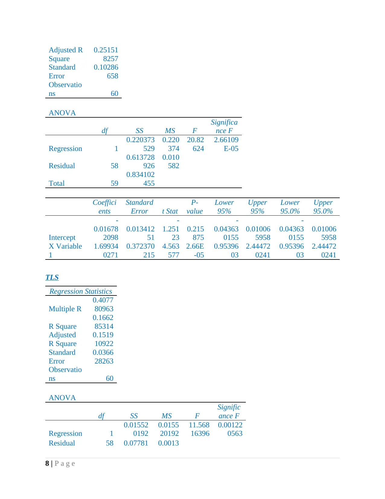
TLS
Regression Statistics
Multiple R
0.4077
80963
R Square
0.1662
85314
Adjusted
R Square
0.1519
10922
Standard
Error
0.0366
28263
Observatio
ns 60
ANOVA
df SS MS F
Signific
ance F
Regression 1
0.01552
0192
0.0155
20192
11.568
16396
0.00122
0563
Residual 58 0.07781 0.0013
8 | P a g e
Square
0.25151
8257
Standard
Error
0.10286
658
Observatio
ns 60
ANOVA
df SS MS F
Significa
nce F
Regression 1
0.220373
529
0.220
374
20.82
624
2.66109
E-05
Residual 58
0.613728
926
0.010
582
Total 59
0.834102
455
Coeffici
ents
Standard
Error t Stat
P-
value
Lower
95%
Upper
95%
Lower
95.0%
Upper
95.0%
Intercept
-
0.01678
2098
0.013412
51
-
1.251
23
0.215
875
-
0.04363
0155
0.01006
5958
-
0.04363
0155
0.01006
5958
X Variable
1
1.69934
0271
0.372370
215
4.563
577
2.66E
-05
0.95396
03
2.44472
0241
0.95396
03
2.44472
0241
TLS
Regression Statistics
Multiple R
0.4077
80963
R Square
0.1662
85314
Adjusted
R Square
0.1519
10922
Standard
Error
0.0366
28263
Observatio
ns 60
ANOVA
df SS MS F
Signific
ance F
Regression 1
0.01552
0192
0.0155
20192
11.568
16396
0.00122
0563
Residual 58 0.07781 0.0013
8 | P a g e
Paraphrase This Document
Need a fresh take? Get an instant paraphrase of this document with our AI Paraphraser
4519 4163
Total 59
0.09333
471
Coeffic
ients
Standar
d Error t Stat
P-
value
Lower
95%
Upper
95%
Lower
95.0%
Upper
95.0%
Intercept
0.0091
64085
0.00477
5865
1.9188
32325
0.0599
31095
-
0.00039
5848
0.0187
24019
-
0.00039
5848
0.0187
24019
X Variable
1
0.4509
71582
0.13259
1889
3.4012
00371
0.0012
20563
0.18556
0079
0.7163
83084
0.18556
0079
0.7163
83084
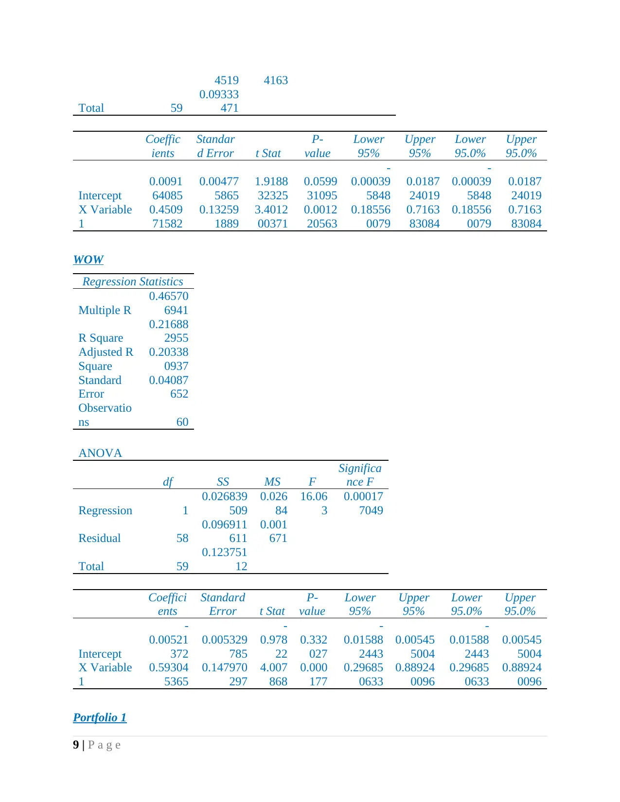
WOW
Regression Statistics
Multiple R
0.46570
6941
R Square
0.21688
2955
Adjusted R
Square
0.20338
0937
Standard
Error
0.04087
652
Observatio
ns 60
ANOVA
df SS MS F
Significa
nce F
Regression 1
0.026839
509
0.026
84
16.06
3
0.00017
7049
Residual 58
0.096911
611
0.001
671
Total 59
0.123751
12
Coeffici
ents
Standard
Error t Stat
P-
value
Lower
95%
Upper
95%
Lower
95.0%
Upper
95.0%
Intercept
-
0.00521
372
0.005329
785
-
0.978
22
0.332
027
-
0.01588
2443
0.00545
5004
-
0.01588
2443
0.00545
5004
X Variable
1
0.59304
5365
0.147970
297
4.007
868
0.000
177
0.29685
0633
0.88924
0096
0.29685
0633
0.88924
0096
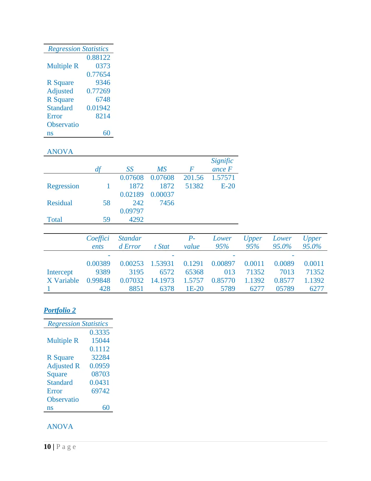
Portfolio 1
9 | P a g e
Total 59
0.09333
471
Coeffic
ients
Standar
d Error t Stat
P-
value
Lower
95%
Upper
95%
Lower
95.0%
Upper
95.0%
Intercept
0.0091
64085
0.00477
5865
1.9188
32325
0.0599
31095
-
0.00039
5848
0.0187
24019
-
0.00039
5848
0.0187
24019
X Variable
1
0.4509
71582
0.13259
1889
3.4012
00371
0.0012
20563
0.18556
0079
0.7163
83084
0.18556
0079
0.7163
83084
WOW
Regression Statistics
Multiple R
0.46570
6941
R Square
0.21688
2955
Adjusted R
Square
0.20338
0937
Standard
Error
0.04087
652
Observatio
ns 60
ANOVA
df SS MS F
Significa
nce F
Regression 1
0.026839
509
0.026
84
16.06
3
0.00017
7049
Residual 58
0.096911
611
0.001
671
Total 59
0.123751
12
Coeffici
ents
Standard
Error t Stat
P-
value
Lower
95%
Upper
95%
Lower
95.0%
Upper
95.0%
Intercept
-
0.00521
372
0.005329
785
-
0.978
22
0.332
027
-
0.01588
2443
0.00545
5004
-
0.01588
2443
0.00545
5004
X Variable
1
0.59304
5365
0.147970
297
4.007
868
0.000
177
0.29685
0633
0.88924
0096
0.29685
0633
0.88924
0096
Portfolio 1
9 | P a g e
Regression Statistics
Multiple R
0.88122
0373
R Square
0.77654
9346
Adjusted
R Square
0.77269
6748
Standard
Error
0.01942
8214
Observatio
ns 60
ANOVA
df SS MS F
Signific
ance F
Regression 1
0.07608
1872
0.07608
1872
201.56
51382
1.57571
E-20
Residual 58
0.02189
242
0.00037
7456
Total 59
0.09797
4292
Coeffici
ents
Standar
d Error t Stat
P-
value
Lower
95%
Upper
95%
Lower
95.0%
Upper
95.0%
Intercept
-
0.00389
9389
0.00253
3195
-
1.53931
6572
0.1291
65368
-
0.00897
013
0.0011
71352
-
0.0089
7013
0.0011
71352
X Variable
1
0.99848
428
0.07032
8851
14.1973
6378
1.5757
1E-20
0.85770
5789
1.1392
6277
0.8577
05789
1.1392
6277
Portfolio 2
Regression Statistics
Multiple R
0.3335
15044
R Square
0.1112
32284
Adjusted R
Square
0.0959
08703
Standard
Error
0.0431
69742
Observatio
ns 60
ANOVA
10 | P a g e
Multiple R
0.88122
0373
R Square
0.77654
9346
Adjusted
R Square
0.77269
6748
Standard
Error
0.01942
8214
Observatio
ns 60
ANOVA
df SS MS F
Signific
ance F
Regression 1
0.07608
1872
0.07608
1872
201.56
51382
1.57571
E-20
Residual 58
0.02189
242
0.00037
7456
Total 59
0.09797
4292
Coeffici
ents
Standar
d Error t Stat
P-
value
Lower
95%
Upper
95%
Lower
95.0%
Upper
95.0%
Intercept
-
0.00389
9389
0.00253
3195
-
1.53931
6572
0.1291
65368
-
0.00897
013
0.0011
71352
-
0.0089
7013
0.0011
71352
X Variable
1
0.99848
428
0.07032
8851
14.1973
6378
1.5757
1E-20
0.85770
5789
1.1392
6277
0.8577
05789
1.1392
6277
Portfolio 2
Regression Statistics
Multiple R
0.3335
15044
R Square
0.1112
32284
Adjusted R
Square
0.0959
08703
Standard
Error
0.0431
69742
Observatio
ns 60
ANOVA
10 | P a g e
df SS MS F
Signific
ance F
Regression 1
0.01352
7872
0.0135
27872
7.2588
96078
0.00921
2299
Residual 58
0.10809
0342
0.0018
63627
Total 59
0.12161
8214
Coeffic
ients
Standar
d Error t Stat
P-
value
Lower
95%
Upper
95%
Lower
95.0%
Upper
95.0%
Intercept
0.0229
19039
0.00562
8792
4.0717
5088
0.0001
43189
0.01165
1788
0.0341
86291
0.0116
51788
0.03418
6291
X Variable
1
0.4210
32262
0.15627
161
2.6942
33857
0.0092
12299
0.10822
0648
0.7338
43875
0.1082
20648
0.73384
3875
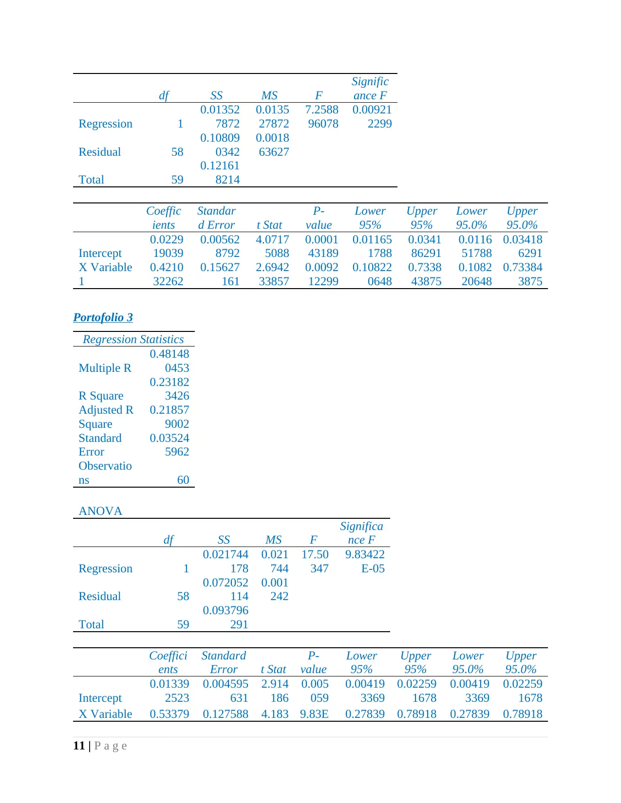
Portofolio 3
Regression Statistics
Multiple R
0.48148
0453
R Square
0.23182
3426
Adjusted R
Square
0.21857
9002
Standard
Error
0.03524
5962
Observatio
ns 60
ANOVA
df SS MS F
Significa
nce F
Regression 1
0.021744
178
0.021
744
17.50
347
9.83422
E-05
Residual 58
0.072052
114
0.001
242
Total 59
0.093796
291
Coeffici
ents
Standard
Error t Stat
P-
value
Lower
95%
Upper
95%
Lower
95.0%
Upper
95.0%
Intercept
0.01339
2523
0.004595
631
2.914
186
0.005
059
0.00419
3369
0.02259
1678
0.00419
3369
0.02259
1678
X Variable 0.53379 0.127588 4.183 9.83E 0.27839 0.78918 0.27839 0.78918
11 | P a g e
Signific
ance F
Regression 1
0.01352
7872
0.0135
27872
7.2588
96078
0.00921
2299
Residual 58
0.10809
0342
0.0018
63627
Total 59
0.12161
8214
Coeffic
ients
Standar
d Error t Stat
P-
value
Lower
95%
Upper
95%
Lower
95.0%
Upper
95.0%
Intercept
0.0229
19039
0.00562
8792
4.0717
5088
0.0001
43189
0.01165
1788
0.0341
86291
0.0116
51788
0.03418
6291
X Variable
1
0.4210
32262
0.15627
161
2.6942
33857
0.0092
12299
0.10822
0648
0.7338
43875
0.1082
20648
0.73384
3875
Portofolio 3
Regression Statistics
Multiple R
0.48148
0453
R Square
0.23182
3426
Adjusted R
Square
0.21857
9002
Standard
Error
0.03524
5962
Observatio
ns 60
ANOVA
df SS MS F
Significa
nce F
Regression 1
0.021744
178
0.021
744
17.50
347
9.83422
E-05
Residual 58
0.072052
114
0.001
242
Total 59
0.093796
291
Coeffici
ents
Standard
Error t Stat
P-
value
Lower
95%
Upper
95%
Lower
95.0%
Upper
95.0%
Intercept
0.01339
2523
0.004595
631
2.914
186
0.005
059
0.00419
3369
0.02259
1678
0.00419
3369
0.02259
1678
X Variable 0.53379 0.127588 4.183 9.83E 0.27839 0.78918 0.27839 0.78918
11 | P a g e
Secure Best Marks with AI Grader
Need help grading? Try our AI Grader for instant feedback on your assignments.
1 2085 051 715 -05 6853 7318 6853 7318
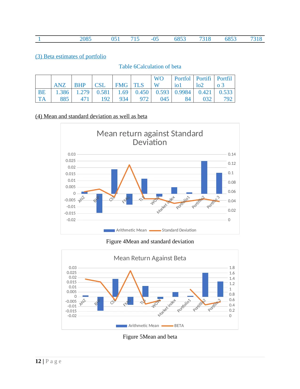
(3) Beta estimates of portfolio
Table 6Calculation of beta
ANZ BHP CSL FMG TLS
WO
W
Portfol
io1
Portifi
lo2
Portfil
o 3
BE
TA
1.386
885
1.279
471
0.581
192
1.69
934
0.450
972
0.593
045
0.9984
84
0.421
032
0.533
792
(4) Mean and standard deviation as well as beta
ANZ
BHP
CSL
FMG
TLS
WOW
Market index
Portfolio1
Portifilo2
Portfilo 3
-0.02
-0.015
-0.01
-0.005
0
0.005
0.01
0.015
0.02
0.025
0.03
0
0.02
0.04
0.06
0.08
0.1
0.12
0.14
Mean return against Standard
Deviation
Arithmetic Mean Standard Deviation
Figure 4Mean and standard deviation
ANZ
BHP
CSL
FMG
TLS
WOW
Market index
Portfolio1
Portifilo2
Portfilo 3
-0.02
-0.015
-0.01
-0.005
0
0.005
0.01
0.015
0.02
0.025
0.03
0
0.2
0.4
0.6
0.8
1
1.2
1.4
1.6
1.8
Mean Return Against Beta
Arithmetic Mean BETA
Figure 5Mean and beta
12 | P a g e
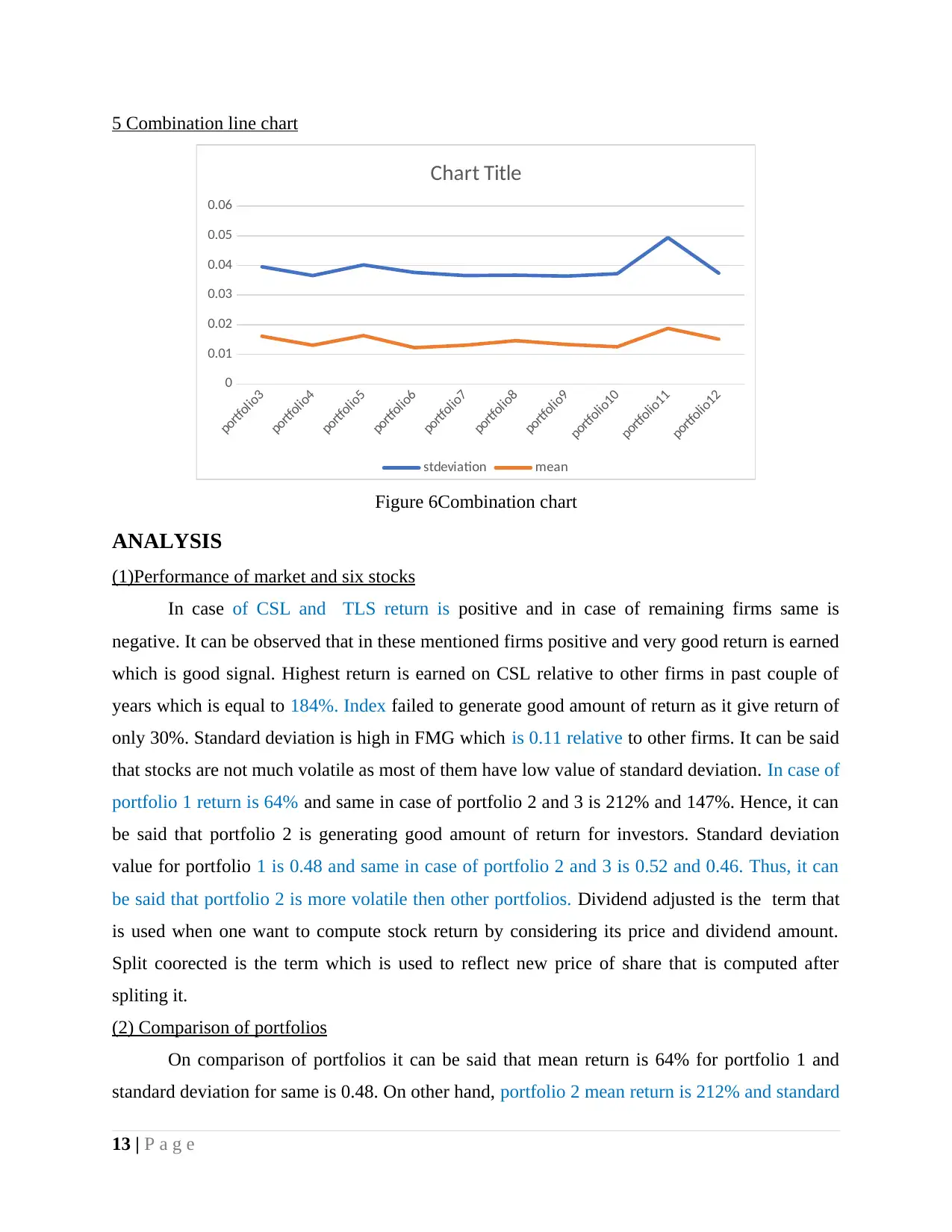
5 Combination line chart
portfolio3
portfolio4
portfolio5
portfolio6
portfolio7
portfolio8
portfolio9
portfolio10
portfolio11
portfolio12
0
0.01
0.02
0.03
0.04
0.05
0.06
Chart Title
stdeviation mean
Figure 6Combination chart
ANALYSIS
(1)Performance of market and six stocks
In case of CSL and TLS return is positive and in case of remaining firms same is
negative. It can be observed that in these mentioned firms positive and very good return is earned
which is good signal. Highest return is earned on CSL relative to other firms in past couple of
years which is equal to 184%. Index failed to generate good amount of return as it give return of
only 30%. Standard deviation is high in FMG which is 0.11 relative to other firms. It can be said
that stocks are not much volatile as most of them have low value of standard deviation. In case of
portfolio 1 return is 64% and same in case of portfolio 2 and 3 is 212% and 147%. Hence, it can
be said that portfolio 2 is generating good amount of return for investors. Standard deviation
value for portfolio 1 is 0.48 and same in case of portfolio 2 and 3 is 0.52 and 0.46. Thus, it can
be said that portfolio 2 is more volatile then other portfolios. Dividend adjusted is the term that
is used when one want to compute stock return by considering its price and dividend amount.
Split coorected is the term which is used to reflect new price of share that is computed after
spliting it.
(2) Comparison of portfolios
On comparison of portfolios it can be said that mean return is 64% for portfolio 1 and
standard deviation for same is 0.48. On other hand, portfolio 2 mean return is 212% and standard
13 | P a g e
deviation is 0.2 followed by return is 147% and standard deviation is 0.46 in case of portoflio 3.
Thus, on the basis of return it can be said that portfolio 2 is one of best option that is available to
investor in terms of return. It can be said that it is one of best option in terms of risk also because
same is not very high in case of same then other portfolios (Bodie, 2013).
(3) Relationship between sharpe ratio portfolio 3,2 and chart ploted in 5th point
Sharpe is related to mentioned portfolios because by using same it can be identified that
apart from risk free rate of return what amount of profit is made for taking each unit of risk on
invested amount. In fifth point combination line is prepared which is reflecting change that
comes in return with change in standard deviation (Meskendahl, 2010). Sharpe ratio reflect same
thing and in this way portfolio and Sharpe ratio are related to each other.
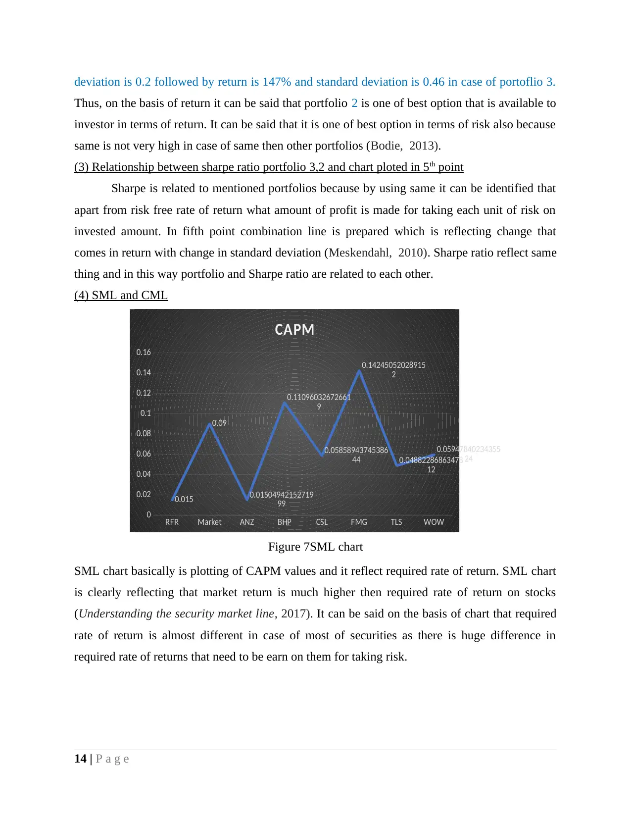
(4) SML and CML
RFR Market ANZ BHP CSL FMG TLS WOW
0
0.02
0.04
0.06
0.08
0.1
0.12
0.14
0.16
0.015
0.09
0.01504942152719
99
0.11096032672661
9
0.05858943745386
44
0.14245052028915
2
0.04882286863478
12
0.05947840234355
24
CAPM
Figure 7SML chart
SML chart basically is plotting of CAPM values and it reflect required rate of return. SML chart
is clearly reflecting that market return is much higher then required rate of return on stocks
(Understanding the security market line, 2017). It can be said on the basis of chart that required
rate of return is almost different in case of most of securities as there is huge difference in
required rate of returns that need to be earn on them for taking risk.
14 | P a g e
Thus, on the basis of return it can be said that portfolio 2 is one of best option that is available to
investor in terms of return. It can be said that it is one of best option in terms of risk also because
same is not very high in case of same then other portfolios (Bodie, 2013).
(3) Relationship between sharpe ratio portfolio 3,2 and chart ploted in 5th point
Sharpe is related to mentioned portfolios because by using same it can be identified that
apart from risk free rate of return what amount of profit is made for taking each unit of risk on
invested amount. In fifth point combination line is prepared which is reflecting change that
comes in return with change in standard deviation (Meskendahl, 2010). Sharpe ratio reflect same
thing and in this way portfolio and Sharpe ratio are related to each other.
(4) SML and CML
RFR Market ANZ BHP CSL FMG TLS WOW
0
0.02
0.04
0.06
0.08
0.1
0.12
0.14
0.16
0.015
0.09
0.01504942152719
99
0.11096032672661
9
0.05858943745386
44
0.14245052028915
2
0.04882286863478
12
0.05947840234355
24
CAPM
Figure 7SML chart
SML chart basically is plotting of CAPM values and it reflect required rate of return. SML chart
is clearly reflecting that market return is much higher then required rate of return on stocks
(Understanding the security market line, 2017). It can be said on the basis of chart that required
rate of return is almost different in case of most of securities as there is huge difference in
required rate of returns that need to be earn on them for taking risk.
14 | P a g e
Paraphrase This Document
Need a fresh take? Get an instant paraphrase of this document with our AI Paraphraser
0.034 0.036 0.038 0.04 0.042 0.044 0.046 0.048 0.05 0.052
0
0.002
0.004
0.006
0.008
0.01
0.012
0.014
0.016
0.018
0.02
Risk and Return Combination Line
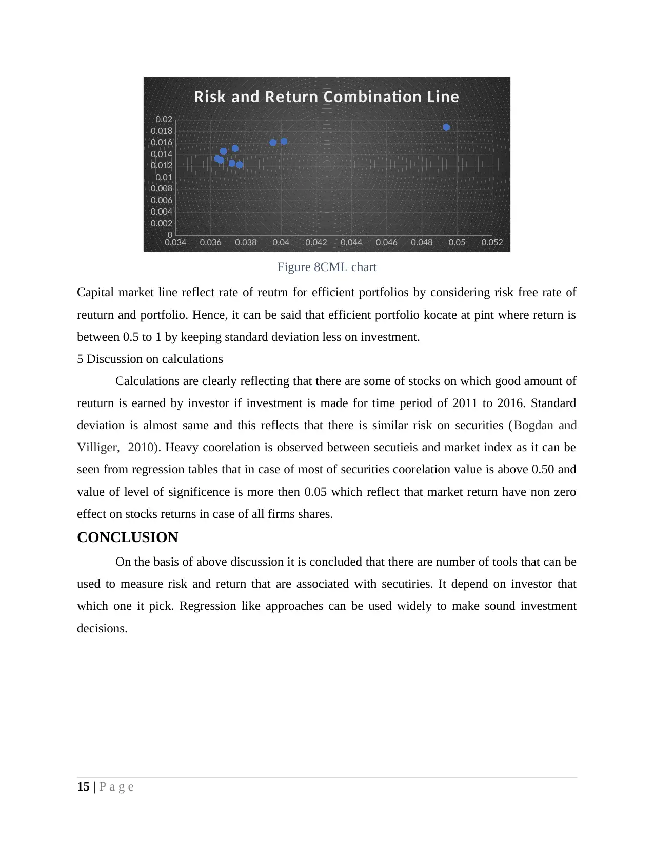
Figure 8CML chart
Capital market line reflect rate of reutrn for efficient portfolios by considering risk free rate of
reuturn and portfolio. Hence, it can be said that efficient portfolio kocate at pint where return is
between 0.5 to 1 by keeping standard deviation less on investment.
5 Discussion on calculations
Calculations are clearly reflecting that there are some of stocks on which good amount of
reuturn is earned by investor if investment is made for time period of 2011 to 2016. Standard
deviation is almost same and this reflects that there is similar risk on securities (Bogdan and
Villiger, 2010). Heavy coorelation is observed between secutieis and market index as it can be
seen from regression tables that in case of most of securities coorelation value is above 0.50 and
value of level of significence is more then 0.05 which reflect that market return have non zero
effect on stocks returns in case of all firms shares.
CONCLUSION
On the basis of above discussion it is concluded that there are number of tools that can be
used to measure risk and return that are associated with secutiries. It depend on investor that
which one it pick. Regression like approaches can be used widely to make sound investment
decisions.
15 | P a g e
0
0.002
0.004
0.006
0.008
0.01
0.012
0.014
0.016
0.018
0.02
Risk and Return Combination Line
Figure 8CML chart
Capital market line reflect rate of reutrn for efficient portfolios by considering risk free rate of
reuturn and portfolio. Hence, it can be said that efficient portfolio kocate at pint where return is
between 0.5 to 1 by keeping standard deviation less on investment.
5 Discussion on calculations
Calculations are clearly reflecting that there are some of stocks on which good amount of
reuturn is earned by investor if investment is made for time period of 2011 to 2016. Standard
deviation is almost same and this reflects that there is similar risk on securities (Bogdan and
Villiger, 2010). Heavy coorelation is observed between secutieis and market index as it can be
seen from regression tables that in case of most of securities coorelation value is above 0.50 and
value of level of significence is more then 0.05 which reflect that market return have non zero
effect on stocks returns in case of all firms shares.
CONCLUSION
On the basis of above discussion it is concluded that there are number of tools that can be
used to measure risk and return that are associated with secutiries. It depend on investor that
which one it pick. Regression like approaches can be used widely to make sound investment
decisions.
15 | P a g e

REFERENCES
Books and Journals
Bodie, Z., (2013). Investments. McGraw-Hill.
Bogdan, B. and Villiger, R., (2010). Introduction. In Valuation in Life Sciences (pp. 1-9).
Springer Berlin Heidelberg.
Meskendahl, S., (2010). The influence of business strategy on project portfolio management and
its success—a conceptual framework. International Journal of Project Management. 28(8).
pp.807-817.
Online
Understanding the security market line, (2017). [Online]. Available through:<
https://courses.lumenlearning.com/boundless-finance/chapter/understanding-the-security-
market-line/>. [Acessed on 12th Octomber 2017].
16 | P a g e
1 out of 21
Related Documents


Your All-in-One AI-Powered Toolkit for Academic Success.
+13062052269
info@desklib.com
Available 24*7 on WhatsApp / Email
![[object Object]](/_next/static/media/star-bottom.7253800d.svg)
Unlock your academic potential
© 2024 | Zucol Services PVT LTD | All rights reserved.