Statistics and Data Analysis Assignment

This assignment focuses on applying statistical concepts to analyze datasets. It includes tasks such as calculating z-scores, determining expected ranks, constructing confidence intervals for proportions, and performing descriptive statistics (mean, median, standard deviation) on quantitative data. The assignment also requires obtaining a dataset, analyzing its composition, and summarizing findings. Finally, there's a section explaining the calculation of expected rate of return and risk using probability and historical data examples.

Business Statistics
Name
Institution
Instructor
Date
1

Section 1
Use the dataset given below you must use the sample allocated to you based on your student
number
https://app.box.com/s/56pb6hqu0ypcg0f3lhy6cl5szt1jgdla
Note that for section 1 the answers are provided so you can check your work, the answers will
not be provided for the other sections.
A) paste in the scatterplot for your sample into your word document and give a simple
comment about the relationship between the variables, (you do not need to submit the
excel file)
Solution
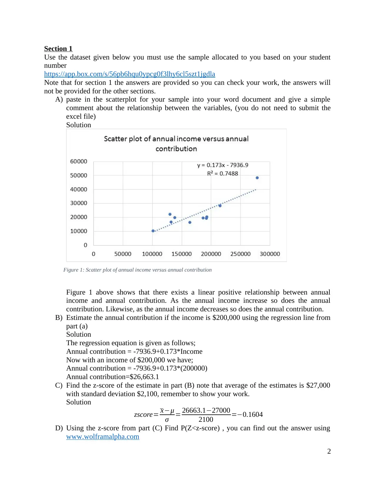
Figure 1: Scatter plot of annual income versus annual contribution
Figure 1 above shows that there exists a linear positive relationship between annual
income and annual contribution. As the annual income increase so does the annual
contribution. Likewise, as the annual income decreases so does the annual contribution.
B) Estimate the annual contribution if the income is $200,000 using the regression line from
part (a)
Solution
The regression equation is given as follows;
Annual contribution = -7936.9+0.173*Income
Now with an income of $200,000 we have;
Annual contribution = -7936.9+0.173*(200000)
Annual contribution=$26,663.1
C) Find the z-score of the estimate in part (B) note that average of the estimates is $27,000
with standard deviation $2,100, remember to show your work.
Solution
zscore= x−μ
σ = 26663.1−27000
2100 =−0.1604
D) Using the z-score from part (C) Find P(Z<z-score) , you can find out the answer using
www.wolframalpha.com
2

for example found the z-score was 1.5 if the z-score is 1.5 type in
P(Z<1.5)
into wolfram alpha.com
Solution
P( Z< zscore)=P( Z <−0.1604)=0.4363
E) If there was a list of 10,000 estimates ranked from lowest to highest, what rank do you
think your estimate would be close to?
Hint: just use the formula
expected rank = P(Z<zscore)*10000, remember to show your work.
Solution
Expected rank =P(Z < zscore )∗10000
Expected rank =0.4363∗10000=4363
Section 2
Use the dataset given below you must use the sample allocated to you based on your student
number
https://app.box.com/s/yvhk3e3oymbs3toy6j5xetid82dsjyz4
A) Use the PivotTable feature in excel to find appropriate summary statistics for your
sample, This will probably require two PivotTables. You should paste both into word,
you do not need the excel file.
Make sure the pivot table (or pivot tables) include the following statistics
*Just considering the high risk (riskier type) investments what is the sample size n1 and
the proportion of high risk investments that made a loss ^p1
*Just considering the low risk (safer type) investments what is the sample size =n2 and
What is the proportion of low risk investments that made a loss ^p2
Solution
Count of made a loss (L or
P)? Column Labels
Row Labels L P
Grand
Total
r 18
5
5 73
s 7
2
0 27
Grand Total 25
7
5 100
The sample size for high risk investment, n1 is 73 while the proportion of high risk
investments that made a loss ^p1 is 18
73 =0.2 466
The sample size for low risk investment, n2 is 30 while the proportion of low risk
investments that made a loss ^p2 is 7
27 =0.2593
3

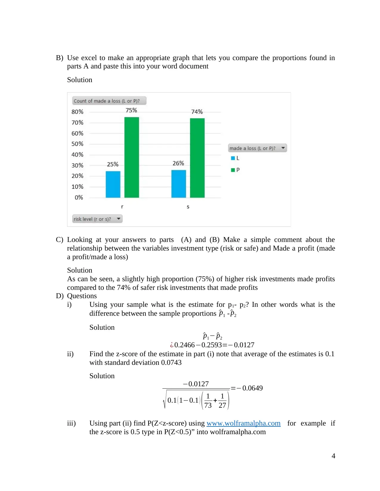
B) Use excel to make an appropriate graph that lets you compare the proportions found in
parts A and paste this into your word document
Solution
C) Looking at your answers to parts (A) and (B) Make a simple comment about the
relationship between the variables investment type (risk or safe) and Made a profit (made
a profit/made a loss)
Solution
As can be seen, a slightly high proportion (75%) of higher risk investments made profits
compared to the 74% of safer risk investments that made profits
D) Questions
i) Using your sample what is the estimate for p1- p2? In other words what is the
difference between the sample proportions ^p1 - ^p2
Solution
^p1− ^p2
¿ 0.2466−0.2593=−0.0127
ii) Find the z-score of the estimate in part (i) note that average of the estimates is 0.1
with standard deviation 0.0743
Solution
−0.0127
√ 0.1 ( 1−0.1 ) ( 1
73 + 1
27 ) =−0.0649
iii) Using part (ii) find P(Z<z-score) using www.wolframalpha.com for example if
the z-score is 0.5 type in P(Z<0.5)” into wolframalpha.com
4

Solution
P( Z ←0.0649)=0.4741
iv) IF there was a list of 4000 estimates ranked from lowest to highest, roughly what
rank do you expect your estimate to have? Hint: just use the formula expected
rank = P(Z<z-score)*4000
Solution
Expected rank = P(Z<z-score)*4000
Expected rank =0.4741*4000=1897
E) Test the claim there is a difference in the proportions use a 5% level of significance
i) State an appropriate H0 and H1
Solution
H0 : ^p1= ^p2
H1 : ^p1 ≠ ^p2
ii) Find the p-value Only using the answers to part (A) and the webpage
http://epitools.ausvet.com.au/content.php?page=z-test-2 Do NOT use any other
method to find the p-value. Do NOT use any other software package such as
SPSS or Analysis tookpak
Solution
Sample 1 Sample 2 Difference
Sample proportion 0.2466 0.2593 0.0127
95% CI (asymptotic) 0.1477 - 0.3455 0.094 - 0.4246 -0.1785 - 0.2039
z-value 0.1
P-value 0.8964
Interpretation
Not significant,
accept null hypothesis that
sample proportions are equal
n by pi n * pi >5, test ok
iii) State whether or not you reject the H0
Solution
We fail to reject the null hypothesis
iv) Give a conclusion in plain English
Solution
There is no significant difference in the proportion of loss for the different types
of investments.
Section 3
Use the dataset given below you must use your own sample
https://app.box.com/s/z0mbtcfsdqxz1rm7rhw3p9sb75aq7174
A) Use the pivot table feature in excel to find appropriate summary statistics for your
sample. The following sample statistics must be found
5

Just considering the low risk investments, what is the sample size n1 , the sample average
return of low risk investments x1 , and the sample standard deviation s1
Just considering the high risk investments , what is the sample size n2 , the sample
average return of high risk investments x2 , and the sample standard deviation s2
Paste the pivot table into the word document you do not need to submit the excel file
Solution
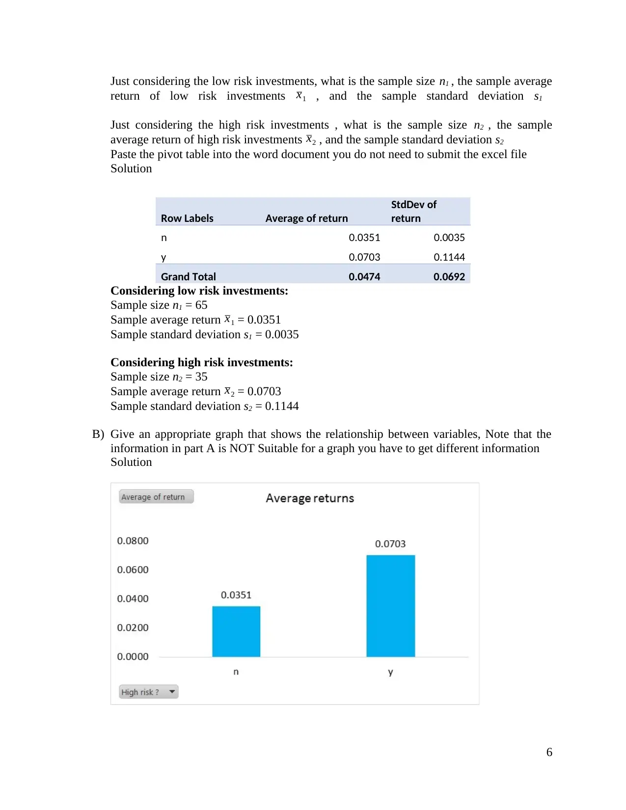
Row Labels Average of return
StdDev of
return
n 0.0351 0.0035
y 0.0703 0.1144
Grand Total 0.0474 0.0692
Considering low risk investments:
Sample size n1 = 65
Sample average return x1 = 0.0351
Sample standard deviation s1 = 0.0035
Considering high risk investments:
Sample size n2 = 35
Sample average return x2 = 0.0703
Sample standard deviation s2 = 0.1144
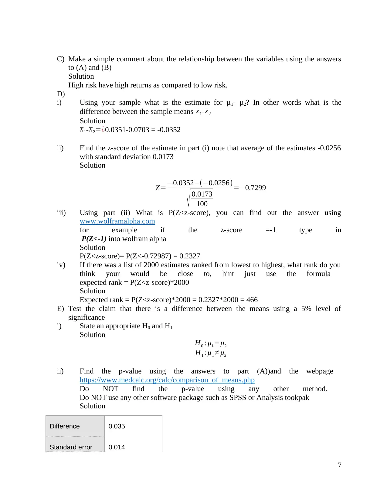
B) Give an appropriate graph that shows the relationship between variables, Note that the
information in part A is NOT Suitable for a graph you have to get different information
Solution
6

C) Make a simple comment about the relationship between the variables using the answers
to (A) and (B)
Solution
High risk have high returns as compared to low risk.
D)
i) Using your sample what is the estimate for μ1- μ2? In other words what is the
difference between the sample means x1- x2
Solution
x1-x2=¿0.0351-0.0703 = -0.0352
ii) Find the z-score of the estimate in part (i) note that average of the estimates -0.0256
with standard deviation 0.0173
Solution
Z=−0.0352−(−0.0256)
√ 0.0173
100
=−0.7299
iii) Using part (ii) What is P(Z<z-score), you can find out the answer using
www.wolframalpha.com
for example if the z-score =-1 type in
P(Z<-1) into wolfram alpha
Solution
P(Z<z-score)= P(Z<-0.72987) = 0.2327
iv) If there was a list of 2000 estimates ranked from lowest to highest, what rank do you
think your would be close to, hint just use the formula
expected rank = P(Z<z-score)*2000
Solution
Expected rank = P(Z<z-score)*2000 = 0.2327*2000 = 466
E) Test the claim that there is a difference between the means using a 5% level of
significance
i) State an appropriate H0 and H1
Solution
H0 : μ1=μ2
H1 : μ1 ≠ μ2
ii) Find the p-value using the answers to part (A))and the webpage
https://www.medcalc.org/calc/comparison_of_means.php
Do NOT find the p-value using any other method.
Do NOT use any other software package such as SPSS or Analysis tookpak
Solution
Difference 0.035
Standard error 0.014
7

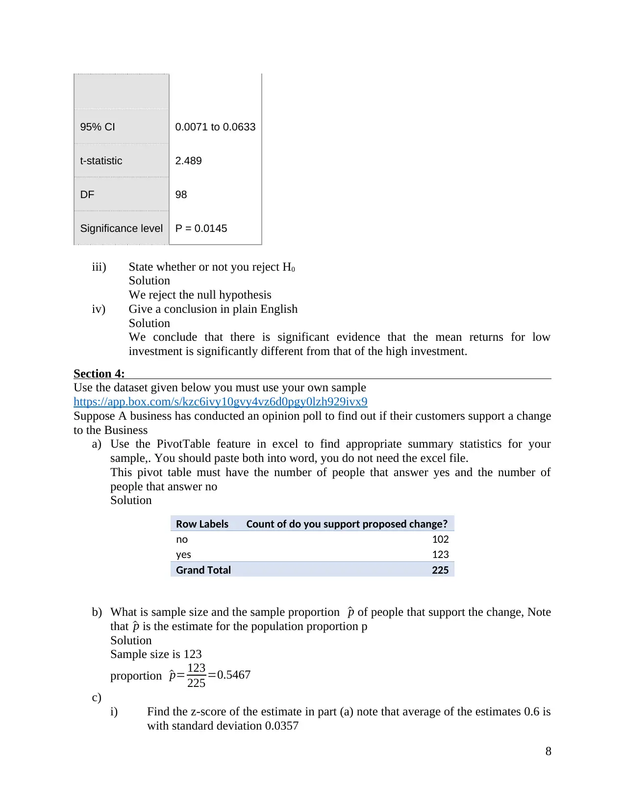
95% CI 0.0071 to 0.0633
t-statistic 2.489
DF 98
Significance level P = 0.0145
iii) State whether or not you reject H0
Solution
We reject the null hypothesis
iv) Give a conclusion in plain English
Solution
We conclude that there is significant evidence that the mean returns for low
investment is significantly different from that of the high investment.
Section 4:
Use the dataset given below you must use your own sample
https://app.box.com/s/kzc6ivy10gvy4vz6d0pgy0lzh929ivx9
Suppose A business has conducted an opinion poll to find out if their customers support a change
to the Business
a) Use the PivotTable feature in excel to find appropriate summary statistics for your
sample,. You should paste both into word, you do not need the excel file.
This pivot table must have the number of people that answer yes and the number of
people that answer no
Solution
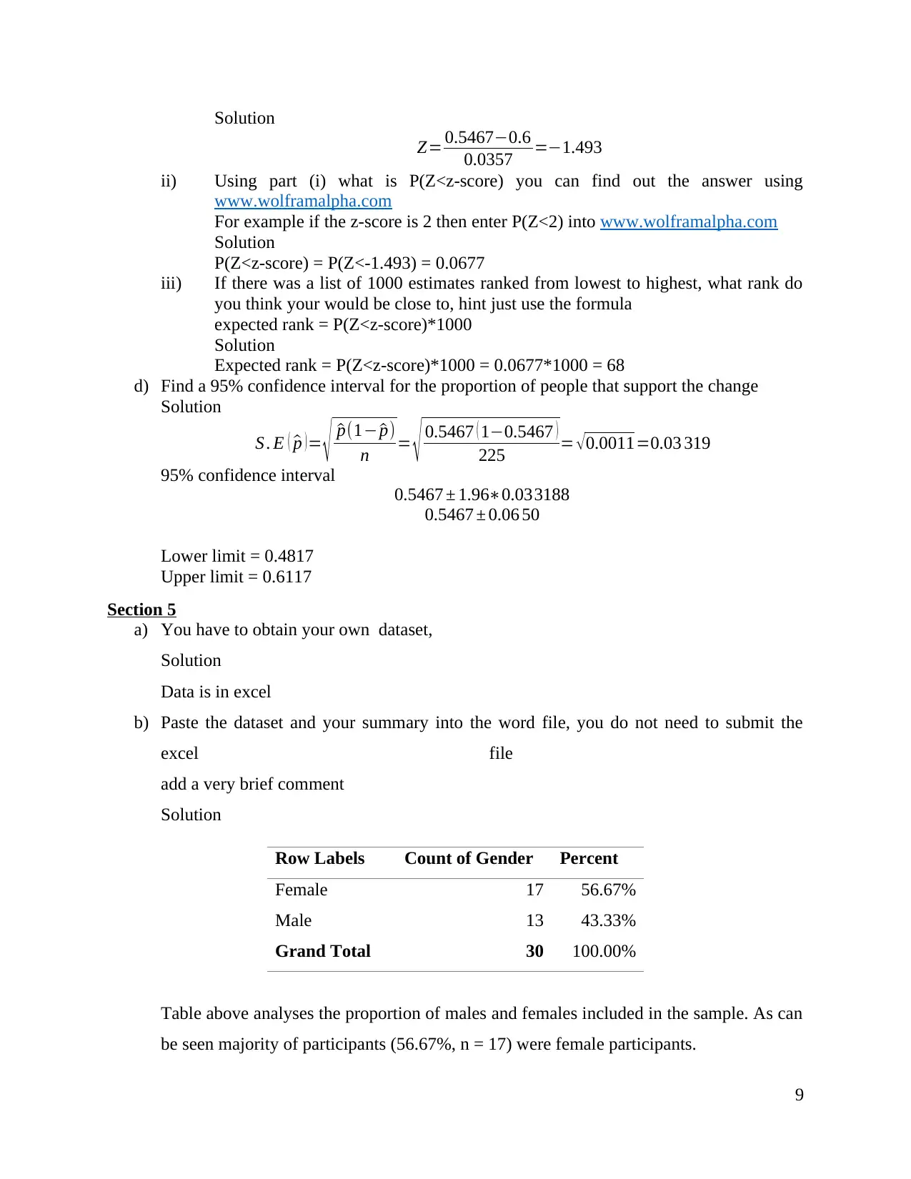
Row Labels Count of do you support proposed change?
no 102
yes 123
Grand Total 225
b) What is sample size and the sample proportion ^p of people that support the change, Note
that ^p is the estimate for the population proportion p
Solution
Sample size is 123
proportion ^p= 123
225 =0.5467
c)
i) Find the z-score of the estimate in part (a) note that average of the estimates 0.6 is
with standard deviation 0.0357
8

Solution
Z= 0.5467−0.6
0.0357 =−1.493
ii) Using part (i) what is P(Z<z-score) you can find out the answer using
www.wolframalpha.com
For example if the z-score is 2 then enter P(Z<2) into www.wolframalpha.com
Solution
P(Z<z-score) = P(Z<-1.493) = 0.0677
iii) If there was a list of 1000 estimates ranked from lowest to highest, what rank do
you think your would be close to, hint just use the formula
expected rank = P(Z<z-score)*1000
Solution
Expected rank = P(Z<z-score)*1000 = 0.0677*1000 = 68
d) Find a 95% confidence interval for the proportion of people that support the change
Solution
S . E ( ^p )= √ ^p(1− ^p)
n = √ 0.5467 ( 1−0.5467 )
225 = √0.0011=0.03 319
95% confidence interval
0.5467 ± 1.96∗0.033188
0.5467 ± 0.06 50
Lower limit = 0.4817
Upper limit = 0.6117
Section 5
a) You have to obtain your own dataset,
Solution
Data is in excel
b) Paste the dataset and your summary into the word file, you do not need to submit the
excel file
add a very brief comment
Solution
Row Labels Count of Gender Percent
Female 17 56.67%
Male 13 43.33%
Grand Total 30 100.00%
Table above analyses the proportion of males and females included in the sample. As can
be seen majority of participants (56.67%, n = 17) were female participants.
9

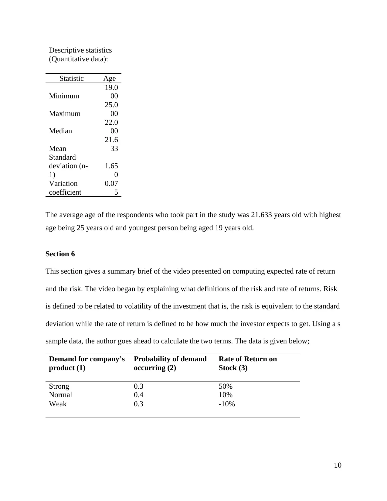
Descriptive statistics
(Quantitative data):
Statistic Age
Minimum
19.0
00
Maximum
25.0
00
Median
22.0
00
Mean
21.6
33
Standard
deviation (n-
1)
1.65
0
Variation
coefficient
0.07
5
The average age of the respondents who took part in the study was 21.633 years old with highest
age being 25 years old and youngest person being aged 19 years old.
Section 6
This section gives a summary brief of the video presented on computing expected rate of return
and the risk. The video began by explaining what definitions of the risk and rate of returns. Risk
is defined to be related to volatility of the investment that is, the risk is equivalent to the standard
deviation while the rate of return is defined to be how much the investor expects to get. Using a s
sample data, the author goes ahead to calculate the two terms. The data is given below;
Demand for company’s
product (1)
Probability of demand
occurring (2)
Rate of Return on
Stock (3)
Strong 0.3 50%
Normal 0.4 10%
Weak 0.3 -10%
10

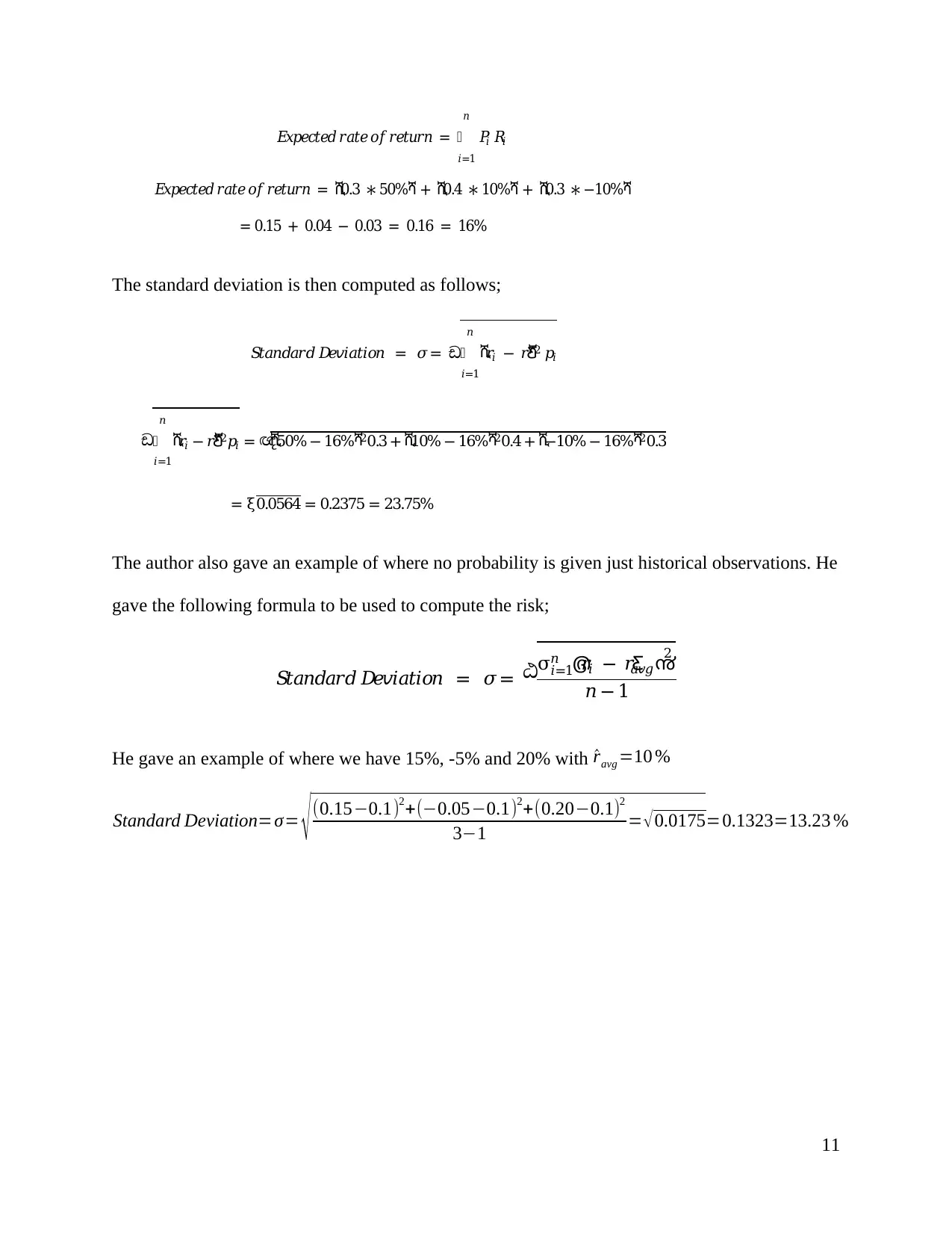
𝐸𝑥𝑝𝑒𝑐𝑡𝑒𝑑 𝑟𝑎𝑡𝑒 𝑜𝑓 𝑟𝑒𝑡𝑢𝑟𝑛 = ෍ 𝑃𝑖 𝑅𝑖
𝑛
𝑖=1
𝐸𝑥𝑝𝑒𝑐𝑡𝑒𝑑 𝑟𝑎𝑡𝑒 𝑜𝑓 𝑟𝑒𝑡𝑢𝑟𝑛 = ሺ0.3 ∗ 50%ሻ + ሺ0.4 ∗ 10%ሻ + ሺ0.3 ∗ −10%ሻ
= 0.15 + 0.04 − 0.03 = 0.16 = 16%
The standard deviation is then computed as follows;
𝑆𝑡𝑎𝑛𝑑𝑎𝑟𝑑 𝐷𝑒𝑣𝑖𝑎𝑡𝑖𝑜𝑛 = 𝜎= ඩ෍ ሺ𝑟𝑖 − 𝑟Ƹሻ2 𝑝𝑖
𝑛
𝑖=1
ඩ෍ ሺ𝑟𝑖 − 𝑟Ƹሻ2𝑝𝑖
𝑛
𝑖=1
= ඥሺ50% − 16%ሻ20.3 + ሺ10% − 16%ሻ20.4 + ሺ−10% − 16%ሻ20.3
= ξ0.0564 = 0.2375 = 23.75%
The author also gave an example of where no probability is given just historical observations. He
gave the following formula to be used to compute the risk;
𝑆𝑡𝑎𝑛𝑑𝑎𝑟𝑑 𝐷𝑒𝑣𝑖𝑎𝑡𝑖𝑜𝑛 = 𝜎= ඨσ ൫𝑟𝑖 − 𝑟Ƹ𝑎𝑣𝑔൯
2𝑛
𝑖=1
𝑛 − 1
He gave an example of where we have 15%, -5% and 20% with ^ravg =10 %
Standard Deviation=σ= √ (0.15−0.1)2+(−0.05−0.1)2+(0.20−0.1)2
3−1 = √ 0.0175=0.1323=13.23 %
11