Business Statistics: Confidence Intervals and Control Charts

This text covers various topics in business statistics such as confidence intervals, control charts, monitoring email systems, insulator problems, shopping downtown, and wine ratings. It includes solved assignments, essays, and dissertations. The text is relevant for students studying business statistics and related courses in colleges and universities.

BUSINESS STATISTICS
STUDENT NAME/ID
[Pick the date]

Question 1 “SHOPPING DOWNTOWN”
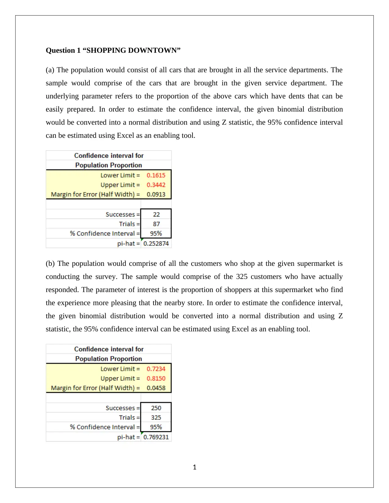
(a) The population would consist of all cars that are brought in all the service departments. The
sample would comprise of the cars that are brought in the given service department. The
underlying parameter refers to the proportion of the above cars which have dents that can be
easily prepared. In order to estimate the confidence interval, the given binomial distribution
would be converted into a normal distribution and using Z statistic, the 95% confidence interval
can be estimated using Excel as an enabling tool.
(b) The population would comprise of all the customers who shop at the given supermarket is
conducting the survey. The sample would comprise of the 325 customers who have actually
responded. The parameter of interest is the proportion of shoppers at this supermarket who find
the experience more pleasing that the nearby store. In order to estimate the confidence interval,
the given binomial distribution would be converted into a normal distribution and using Z
statistic, the 95% confidence interval can be estimated using Excel as an enabling tool.
1

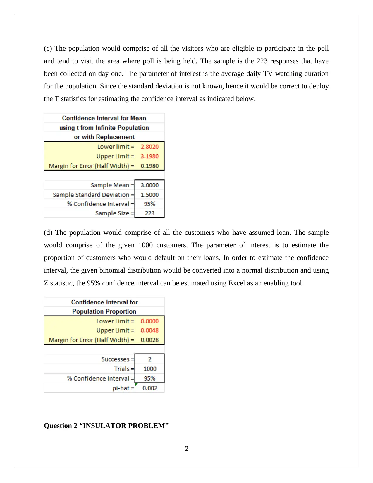
(c) The population would comprise of all the visitors who are eligible to participate in the poll
and tend to visit the area where poll is being held. The sample is the 223 responses that have
been collected on day one. The parameter of interest is the average daily TV watching duration
for the population. Since the standard deviation is not known, hence it would be correct to deploy
the T statistics for estimating the confidence interval as indicated below.
(d) The population would comprise of all the customers who have assumed loan. The sample
would comprise of the given 1000 customers. The parameter of interest is to estimate the
proportion of customers who would default on their loans. In order to estimate the confidence
interval, the given binomial distribution would be converted into a normal distribution and using
Z statistic, the 95% confidence interval can be estimated using Excel as an enabling tool
Question 2 “INSULATOR PROBLEM”
2

Desired thickness = 250 micron
95% of chips are having thickness between 247 microns to 253 microns.
12 sample chips has been taken for 40 days which means the total sample size = 480 chips
(a) Sample size condition: Sample size must be greater than the 10 times absolute value of
kurtosis.
The kurtosis of the given thickness data has been determined through = KURT() which comes
out to be 1.132217.
Now,
¿ 10∗1.132217=11.32217
Condition, sample size > 10 times |K|
¿ 12>11.32217
Therefore, it can be said that sample size condition is met.
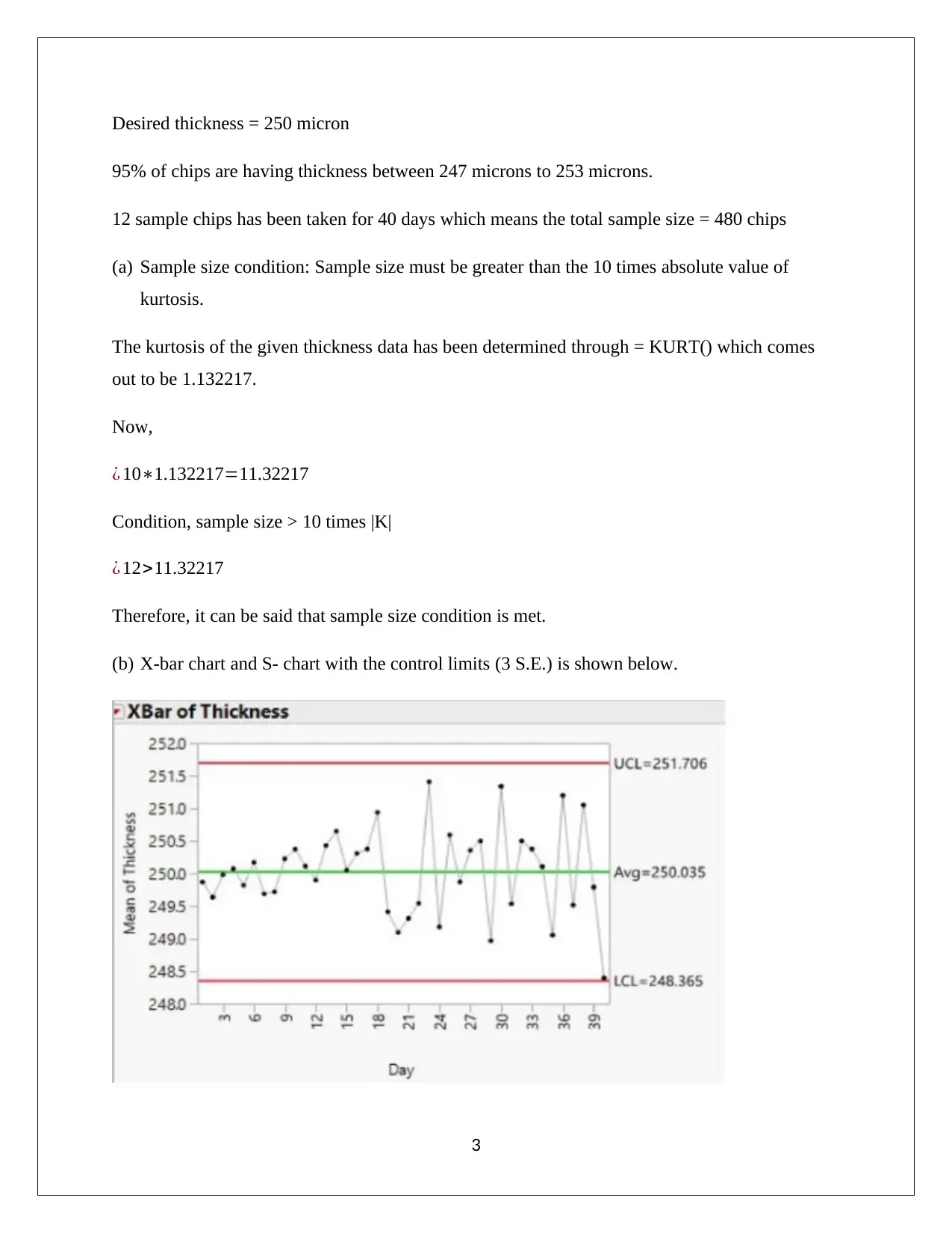
(b) X-bar chart and S- chart with the control limits (3 S.E.) is shown below.
3

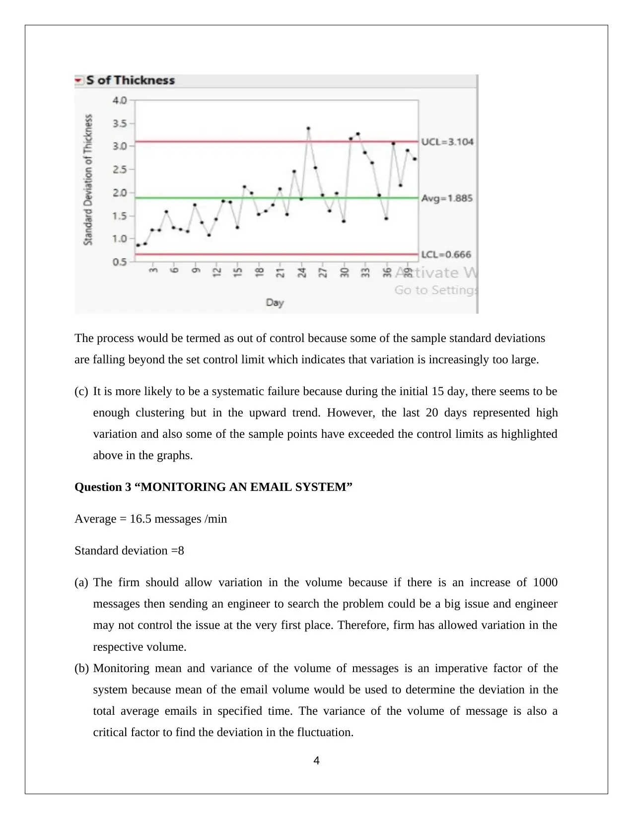
The process would be termed as out of control because some of the sample standard deviations
are falling beyond the set control limit which indicates that variation is increasingly too large.
(c) It is more likely to be a systematic failure because during the initial 15 day, there seems to be
enough clustering but in the upward trend. However, the last 20 days represented high
variation and also some of the sample points have exceeded the control limits as highlighted
above in the graphs.
Question 3 “MONITORING AN EMAIL SYSTEM”
Average = 16.5 messages /min
Standard deviation =8
(a) The firm should allow variation in the volume because if there is an increase of 1000
messages then sending an engineer to search the problem could be a big issue and engineer
may not control the issue at the very first place. Therefore, firm has allowed variation in the
respective volume.
(b) Monitoring mean and variance of the volume of messages is an imperative factor of the
system because mean of the email volume would be used to determine the deviation in the
total average emails in specified time. The variance of the volume of message is also a
critical factor to find the deviation in the fluctuation.
4

(c) It is apparent that failing to check a problem can be a serious issue for the system and further,
the cost to check is quite minimal and hence, the problem should be checked. The cost for
type I error is very low as compared with the cost of type II error and hence, the system can
easily afford the cost incurred for type I error. The recommend value for type I error would
be high such as ∝=0.10 .
(d) Advantage of grouping the data for a 15 min period would allow the use of normal
distribution. Hence, the mean would be a critical factor to determine any deviation in the
mean number of emails. Further, the disadvantage is to find a minimum sample before
representing an issue in the system.
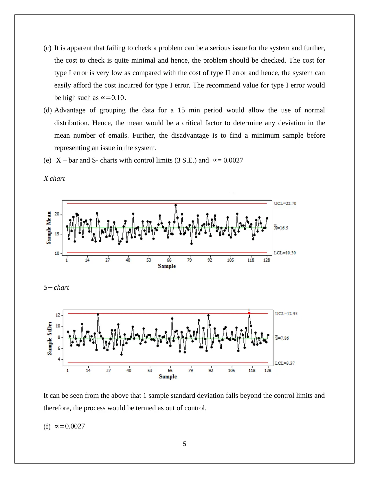
(e) X – bar and S- charts with control limits (3 S.E.) and ∝= 0.0027
X ¯chart
S−chart
It can be seen from the above that 1 sample standard deviation falls beyond the control limits and
therefore, the process would be termed as out of control.
(f) ∝=0.0027
5

Control limits z=± 3 S . E .
The probability that sample average will go out of the limits = 0.0027
Probability that sample average will not cross the limits = 1- 0.0027 = 0.9973
Probability that system remains would be under control for four days whereas the control charts
signal an issue = 1 – (0.9973) ^4 = 0.293
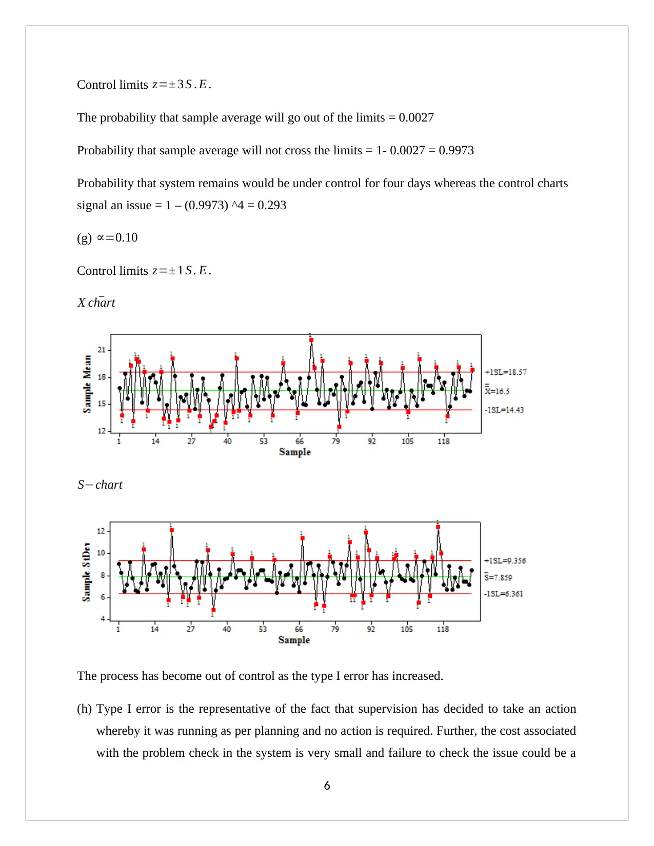
(g) ∝=0.10
Control limits z=± 1 S . E .
X ¯chart
S−chart
The process has become out of control as the type I error has increased.
(h) Type I error is the representative of the fact that supervision has decided to take an action
whereby it was running as per planning and no action is required. Further, the cost associated
with the problem check in the system is very small and failure to check the issue could be a
6

serious problem. The cost of type I error is lesser than the cost of type II error and therefore,
increasing the type I error would reduce the probability of type II error in system.
Question “Wine”
(a) The rating might meet the requisite condition because the confidence interval for the two
sample data 2000 and 2001 vintage are numerical. However, the method of selecting the
sample from population is not known which means the condition for the rating may not
satisfy. Further, the test also allows the two populations with different variances which
indicate that bottles might offer good selection. The two samples represent that data 2000 and
2001 provide different means and hence, the flaw of sampling is considered fatal.
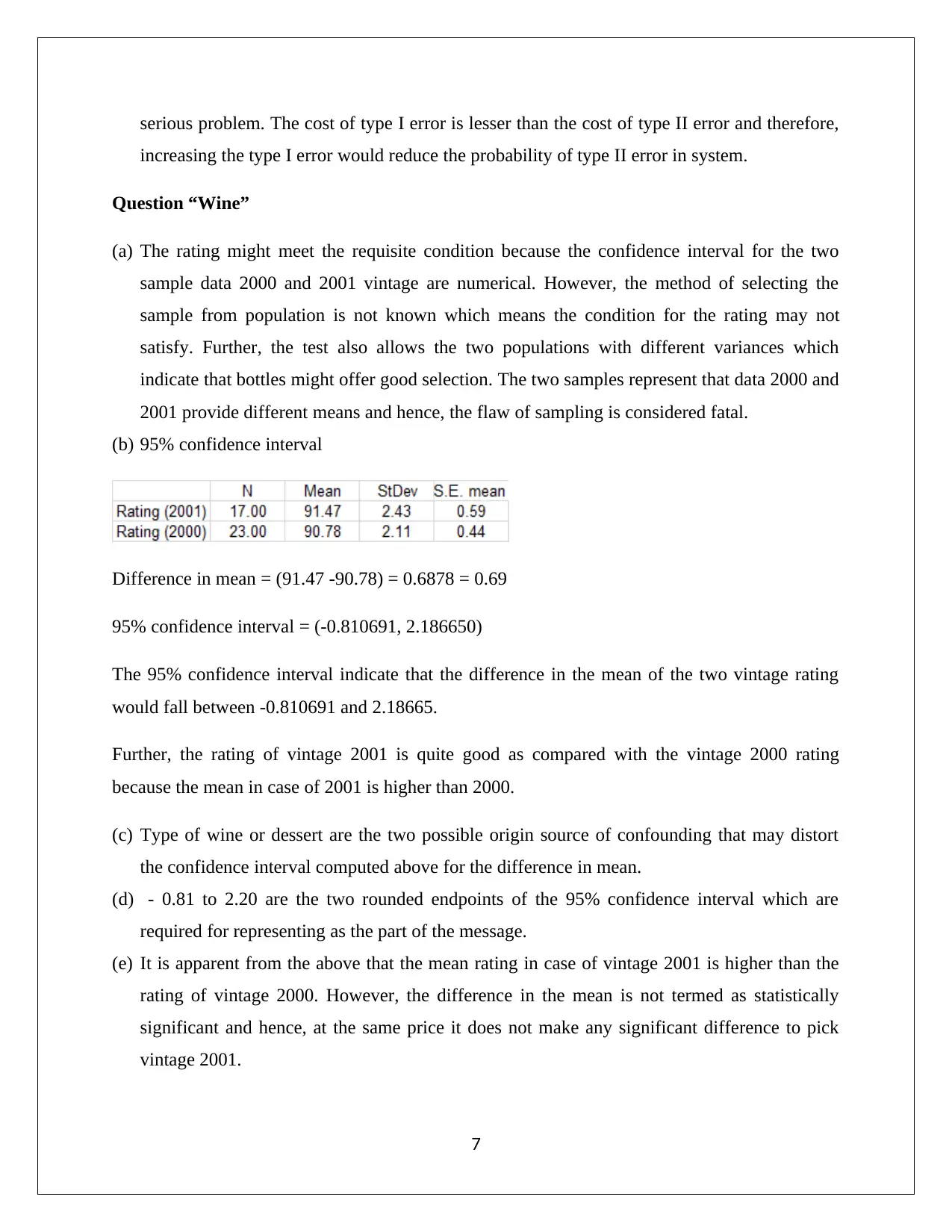
(b) 95% confidence interval
Difference in mean = (91.47 -90.78) = 0.6878 = 0.69
95% confidence interval = (-0.810691, 2.186650)
The 95% confidence interval indicate that the difference in the mean of the two vintage rating
would fall between -0.810691 and 2.18665.
Further, the rating of vintage 2001 is quite good as compared with the vintage 2000 rating
because the mean in case of 2001 is higher than 2000.
(c) Type of wine or dessert are the two possible origin source of confounding that may distort
the confidence interval computed above for the difference in mean.
(d) - 0.81 to 2.20 are the two rounded endpoints of the 95% confidence interval which are
required for representing as the part of the message.
(e) It is apparent from the above that the mean rating in case of vintage 2001 is higher than the
rating of vintage 2000. However, the difference in the mean is not termed as statistically
significant and hence, at the same price it does not make any significant difference to pick
vintage 2001.
7

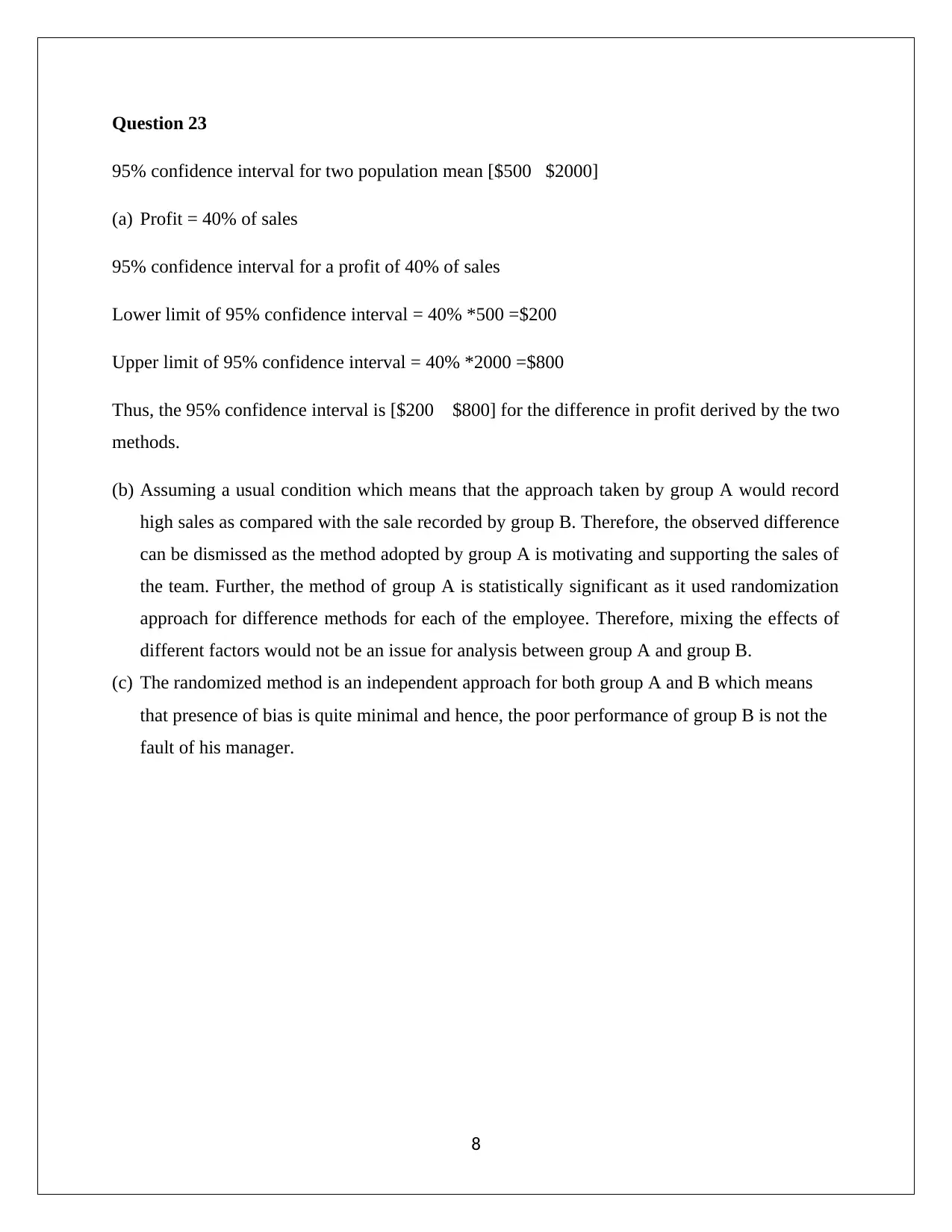
Question 23
95% confidence interval for two population mean [$500 $2000]
(a) Profit = 40% of sales
95% confidence interval for a profit of 40% of sales
Lower limit of 95% confidence interval = 40% *500 =$200
Upper limit of 95% confidence interval = 40% *2000 =$800
Thus, the 95% confidence interval is [$200 $800] for the difference in profit derived by the two
methods.
(b) Assuming a usual condition which means that the approach taken by group A would record
high sales as compared with the sale recorded by group B. Therefore, the observed difference
can be dismissed as the method adopted by group A is motivating and supporting the sales of
the team. Further, the method of group A is statistically significant as it used randomization
approach for difference methods for each of the employee. Therefore, mixing the effects of
different factors would not be an issue for analysis between group A and group B.
(c) The randomized method is an independent approach for both group A and B which means
that presence of bias is quite minimal and hence, the poor performance of group B is not the
fault of his manager.
8