Snack Food Preference Survey

This assignment analyzes the results of a student-conducted survey on snack food preferences. The survey aimed to determine consumer preference between two versions of a snack food, assess product liking, and gather demographic information such as age and gender. The findings revealed that while men slightly preferred one version over women, the difference was not statistically significant. The assignment recommends further market research and targeted advertising strategies based on these results.

Business Statistics
Name
Institution
Instructor
Date
1

Section 1
Use the dataset given below you must use the sample allocated to you based on your student
number
https://app.box.com/s/56pb6hqu0ypcg0f3lhy6cl5szt1jgdla
Note that for section 1 the answers are provided so you can check your work, the answers will
not be provided for the other sections.
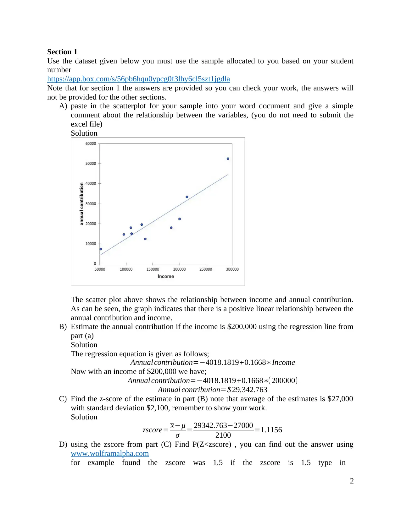
A) paste in the scatterplot for your sample into your word document and give a simple
comment about the relationship between the variables, (you do not need to submit the
excel file)
Solution
The scatter plot above shows the relationship between income and annual contribution.
As can be seen, the graph indicates that there is a positive linear relationship between the
annual contribution and income.
B) Estimate the annual contribution if the income is $200,000 using the regression line from
part (a)
Solution
The regression equation is given as follows;
Annual contribution=−4018.1819+0.1668∗Income
Now with an income of $200,000 we have;
Annual contribution=−4018.1819+0.1668∗(200000)
Annual contribution=$ 29,342.763
C) Find the z-score of the estimate in part (B) note that average of the estimates is $27,000
with standard deviation $2,100, remember to show your work.
Solution
zscore= x−μ
σ = 29342.763−27000
2100 =1.1156
D) using the zscore from part (C) Find P(Z<zscore) , you can find out the answer using
www.wolframalpha.com
for example found the zscore was 1.5 if the zscore is 1.5 type in
2

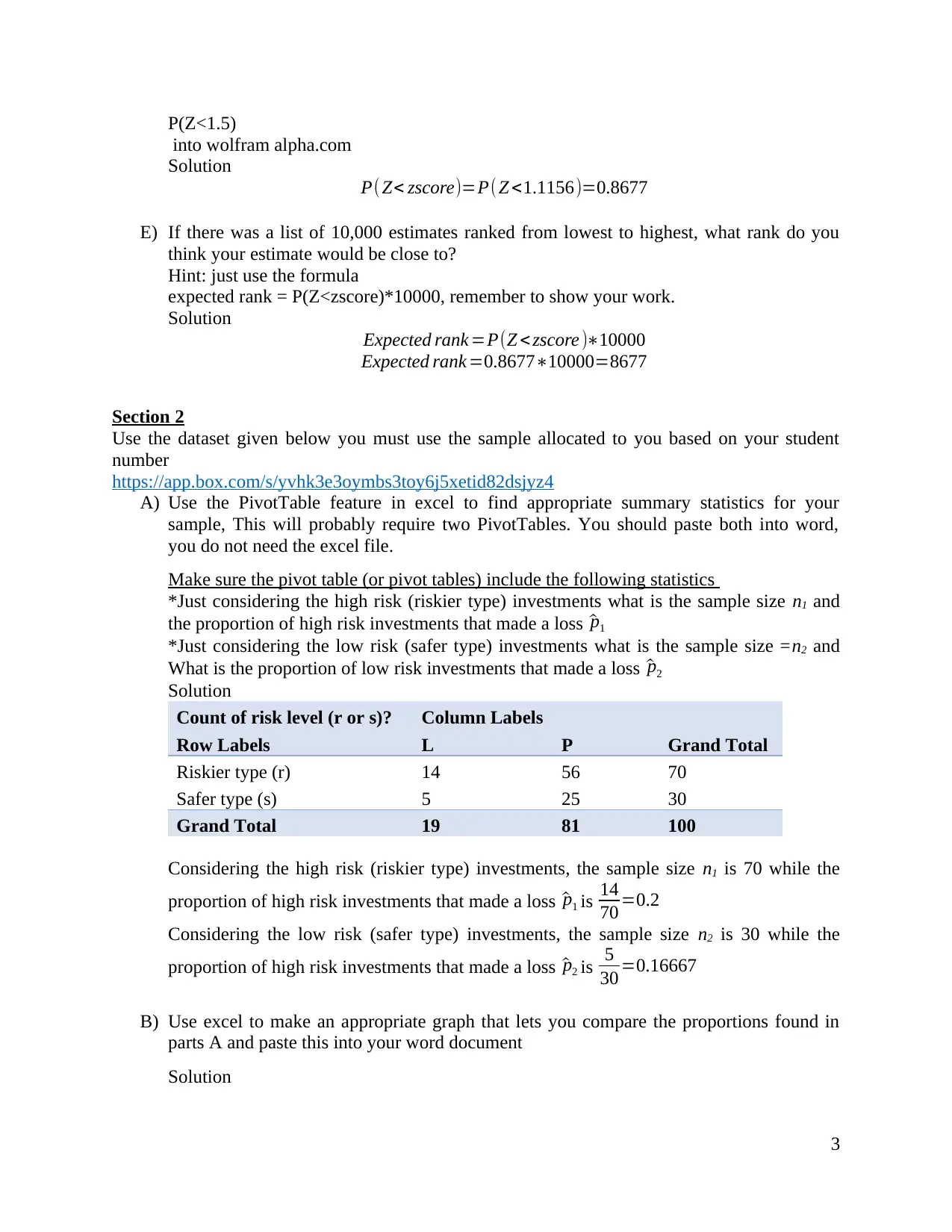
P(Z<1.5)
into wolfram alpha.com
Solution
P( Z< zscore)=P( Z <1.1156)=0.8677
E) If there was a list of 10,000 estimates ranked from lowest to highest, what rank do you
think your estimate would be close to?
Hint: just use the formula
expected rank = P(Z<zscore)*10000, remember to show your work.
Solution
Expected rank =P(Z < zscore )∗10000
Expected rank =0.8677∗10000=8677
Section 2
Use the dataset given below you must use the sample allocated to you based on your student
number
https://app.box.com/s/yvhk3e3oymbs3toy6j5xetid82dsjyz4
A) Use the PivotTable feature in excel to find appropriate summary statistics for your
sample, This will probably require two PivotTables. You should paste both into word,
you do not need the excel file.
Make sure the pivot table (or pivot tables) include the following statistics
*Just considering the high risk (riskier type) investments what is the sample size n1 and
the proportion of high risk investments that made a loss ^p1
*Just considering the low risk (safer type) investments what is the sample size =n2 and
What is the proportion of low risk investments that made a loss ^p2
Solution
Count of risk level (r or s)? Column Labels
Row Labels L P Grand Total
Riskier type (r) 14 56 70
Safer type (s) 5 25 30
Grand Total 19 81 100
Considering the high risk (riskier type) investments, the sample size n1 is 70 while the
proportion of high risk investments that made a loss ^p1 is 14
70 =0.2
Considering the low risk (safer type) investments, the sample size n2 is 30 while the
proportion of high risk investments that made a loss ^p2 is 5
30 =0.16667
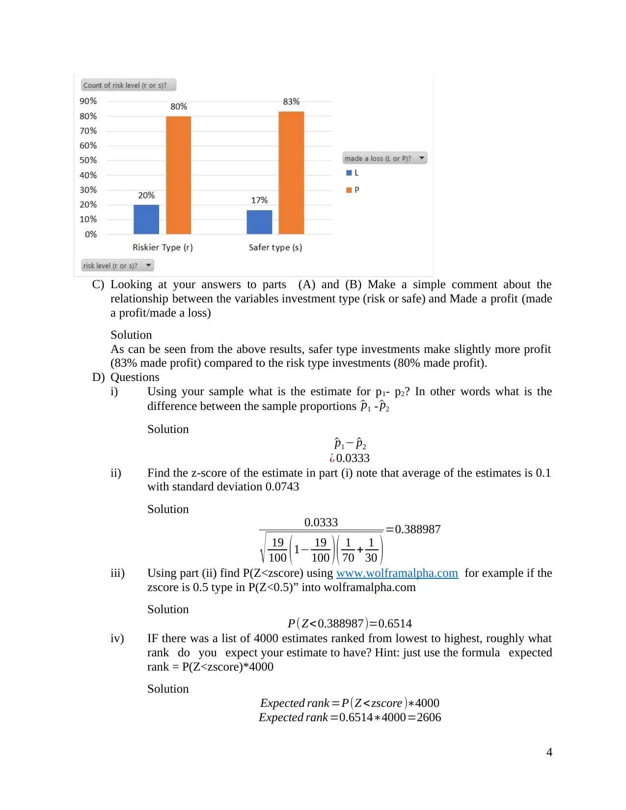
B) Use excel to make an appropriate graph that lets you compare the proportions found in
parts A and paste this into your word document
Solution
3

C) Looking at your answers to parts (A) and (B) Make a simple comment about the
relationship between the variables investment type (risk or safe) and Made a profit (made
a profit/made a loss)
Solution
As can be seen from the above results, safer type investments make slightly more profit
(83% made profit) compared to the risk type investments (80% made profit).
D) Questions
i) Using your sample what is the estimate for p1- p2? In other words what is the
difference between the sample proportions ^p1 - ^p2
Solution
^p1− ^p2
¿ 0.0333
ii) Find the z-score of the estimate in part (i) note that average of the estimates is 0.1
with standard deviation 0.0743
Solution
0.0333
√ 19
100 (1− 19
100 )( 1
70 + 1
30 )=0.388987
iii) Using part (ii) find P(Z<zscore) using www.wolframalpha.com for example if the
zscore is 0.5 type in P(Z<0.5)” into wolframalpha.com
Solution
P(Z< 0.388987)=0.6514
iv) IF there was a list of 4000 estimates ranked from lowest to highest, roughly what
rank do you expect your estimate to have? Hint: just use the formula expected
rank = P(Z<zscore)*4000
Solution
Expected rank =P(Z <zscore )∗4000
Expected rank =0.6514∗4000=2606
4

E) Test the claim there is a difference in the proportions use a 5% level of significance
i) State an appropriate H0 and H1
Solution
H0 : ^p1= ^p2
H1 : ^p1 ≠ ^p2
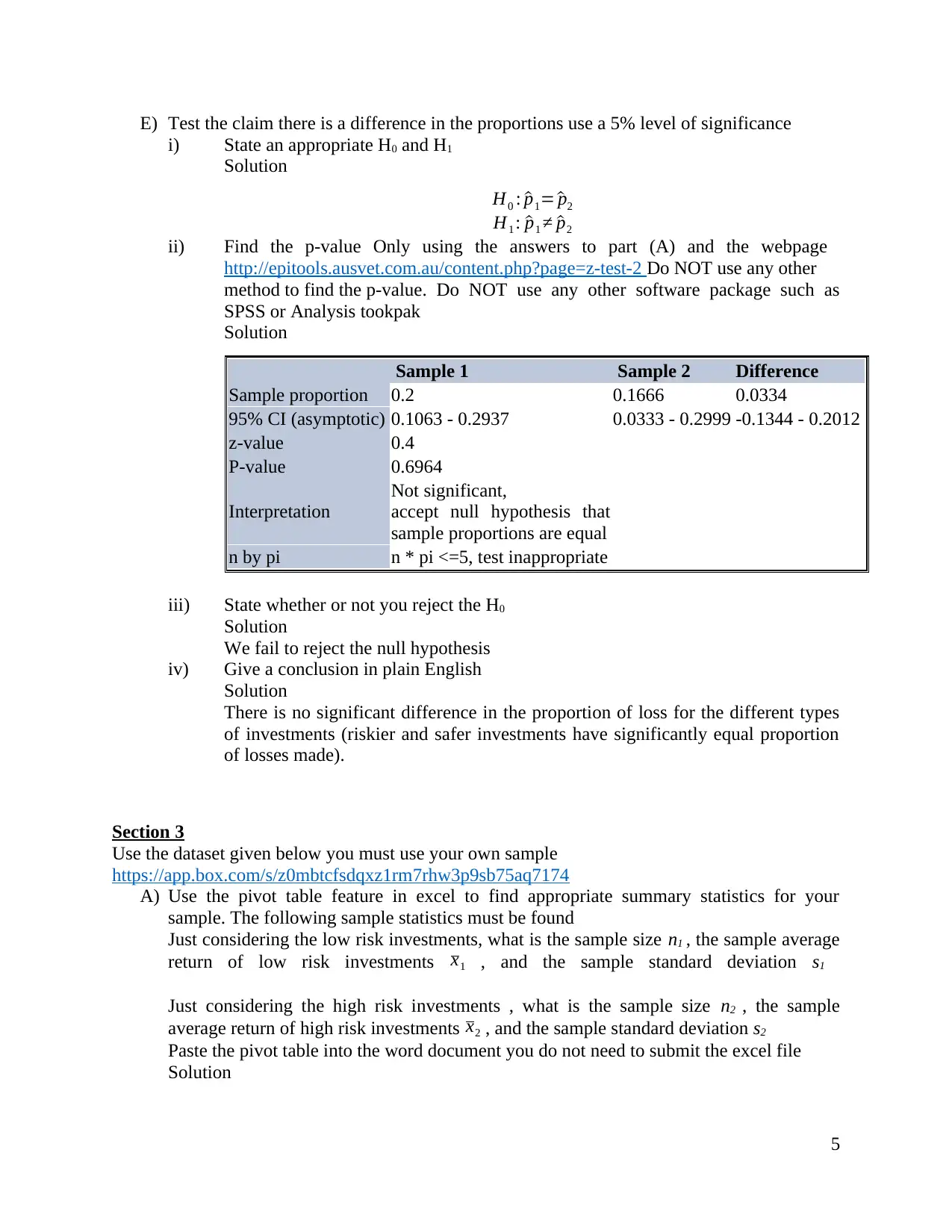
ii) Find the p-value Only using the answers to part (A) and the webpage
http://epitools.ausvet.com.au/content.php?page=z-test-2 Do NOT use any other
method to find the p-value. Do NOT use any other software package such as
SPSS or Analysis tookpak
Solution
Sample 1 Sample 2 Difference
Sample proportion 0.2 0.1666 0.0334
95% CI (asymptotic) 0.1063 - 0.2937 0.0333 - 0.2999 -0.1344 - 0.2012
z-value 0.4
P-value 0.6964
Interpretation
Not significant,
accept null hypothesis that
sample proportions are equal
n by pi n * pi <=5, test inappropriate
iii) State whether or not you reject the H0
Solution
We fail to reject the null hypothesis
iv) Give a conclusion in plain English
Solution
There is no significant difference in the proportion of loss for the different types
of investments (riskier and safer investments have significantly equal proportion
of losses made).
Section 3
Use the dataset given below you must use your own sample
https://app.box.com/s/z0mbtcfsdqxz1rm7rhw3p9sb75aq7174
A) Use the pivot table feature in excel to find appropriate summary statistics for your
sample. The following sample statistics must be found
Just considering the low risk investments, what is the sample size n1 , the sample average
return of low risk investments x1 , and the sample standard deviation s1
Just considering the high risk investments , what is the sample size n2 , the sample
average return of high risk investments x2 , and the sample standard deviation s2
Paste the pivot table into the word document you do not need to submit the excel file
Solution
5

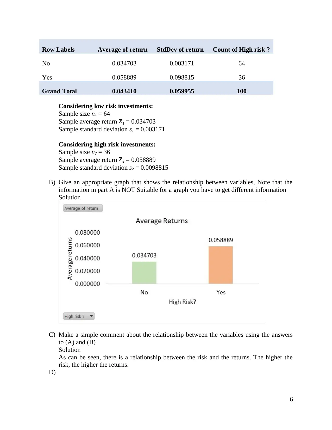
Row Labels Average of return StdDev of return Count of High risk ?
No 0.034703 0.003171 64
Yes 0.058889 0.098815 36
Grand Total 0.043410 0.059955 100
Considering low risk investments:
Sample size n1 = 64
Sample average return x1 = 0.034703
Sample standard deviation s1 = 0.003171
Considering high risk investments:
Sample size n2 = 36
Sample average return x2 = 0.058889
Sample standard deviation s2 = 0.0098815
B) Give an appropriate graph that shows the relationship between variables, Note that the
information in part A is NOT Suitable for a graph you have to get different information
Solution
C) Make a simple comment about the relationship between the variables using the answers
to (A) and (B)
Solution
As can be seen, there is a relationship between the risk and the returns. The higher the
risk, the higher the returns.
D)
6

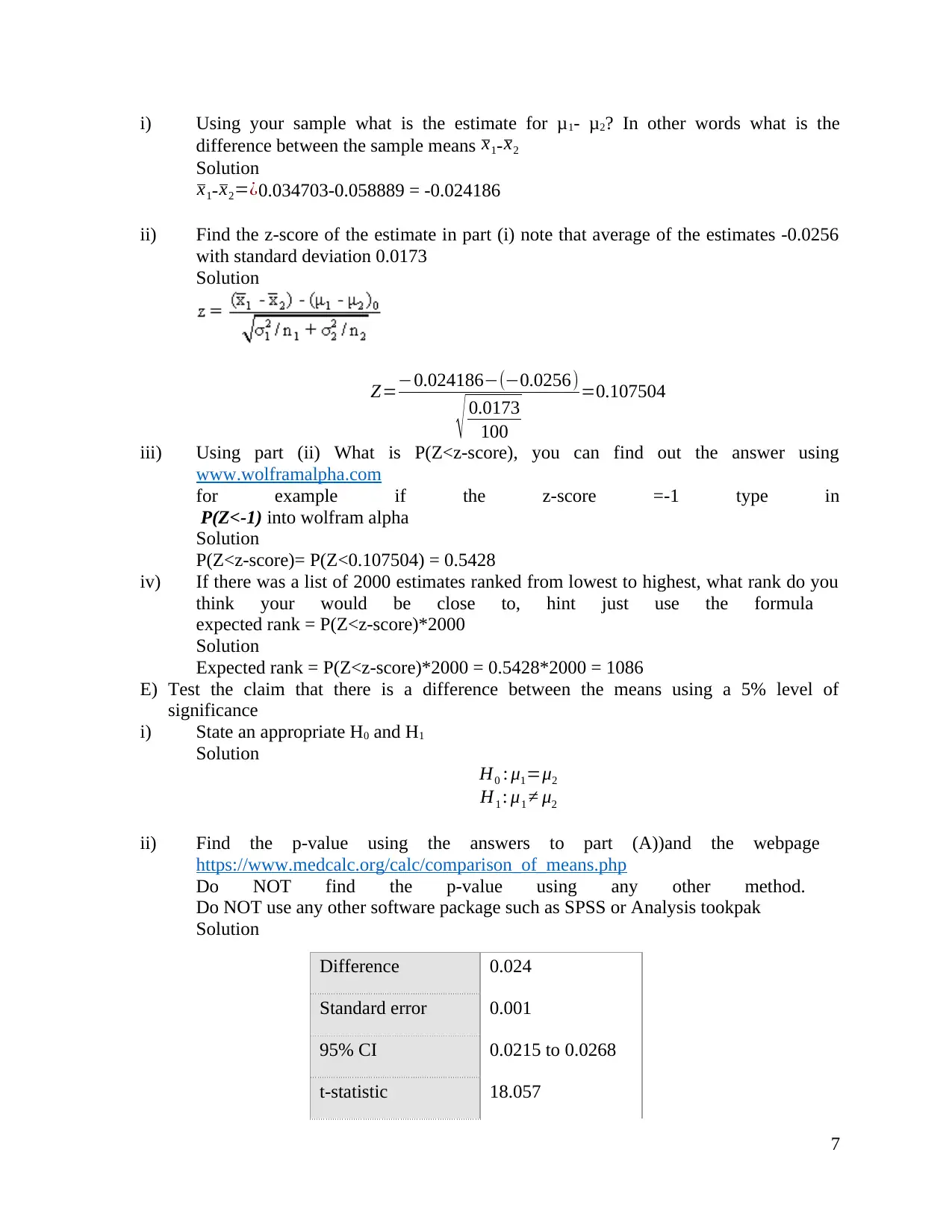
i) Using your sample what is the estimate for μ1- μ2? In other words what is the
difference between the sample means x1- x2
Solution
x1-x2=¿0.034703-0.058889 = -0.024186
ii) Find the z-score of the estimate in part (i) note that average of the estimates -0.0256
with standard deviation 0.0173
Solution
Z=−0.024186−(−0.0256)
√ 0.0173
100
=0.107504
iii) Using part (ii) What is P(Z<z-score), you can find out the answer using
www.wolframalpha.com
for example if the z-score =-1 type in
P(Z<-1) into wolfram alpha
Solution
P(Z<z-score)= P(Z<0.107504) = 0.5428
iv) If there was a list of 2000 estimates ranked from lowest to highest, what rank do you
think your would be close to, hint just use the formula
expected rank = P(Z<z-score)*2000
Solution
Expected rank = P(Z<z-score)*2000 = 0.5428*2000 = 1086
E) Test the claim that there is a difference between the means using a 5% level of
significance
i) State an appropriate H0 and H1
Solution
H0 : μ1=μ2
H1 : μ1 ≠ μ2
ii) Find the p-value using the answers to part (A))and the webpage
https://www.medcalc.org/calc/comparison_of_means.php
Do NOT find the p-value using any other method.
Do NOT use any other software package such as SPSS or Analysis tookpak
Solution
Difference 0.024
Standard error 0.001
95% CI 0.0215 to 0.0268
t-statistic 18.057
7

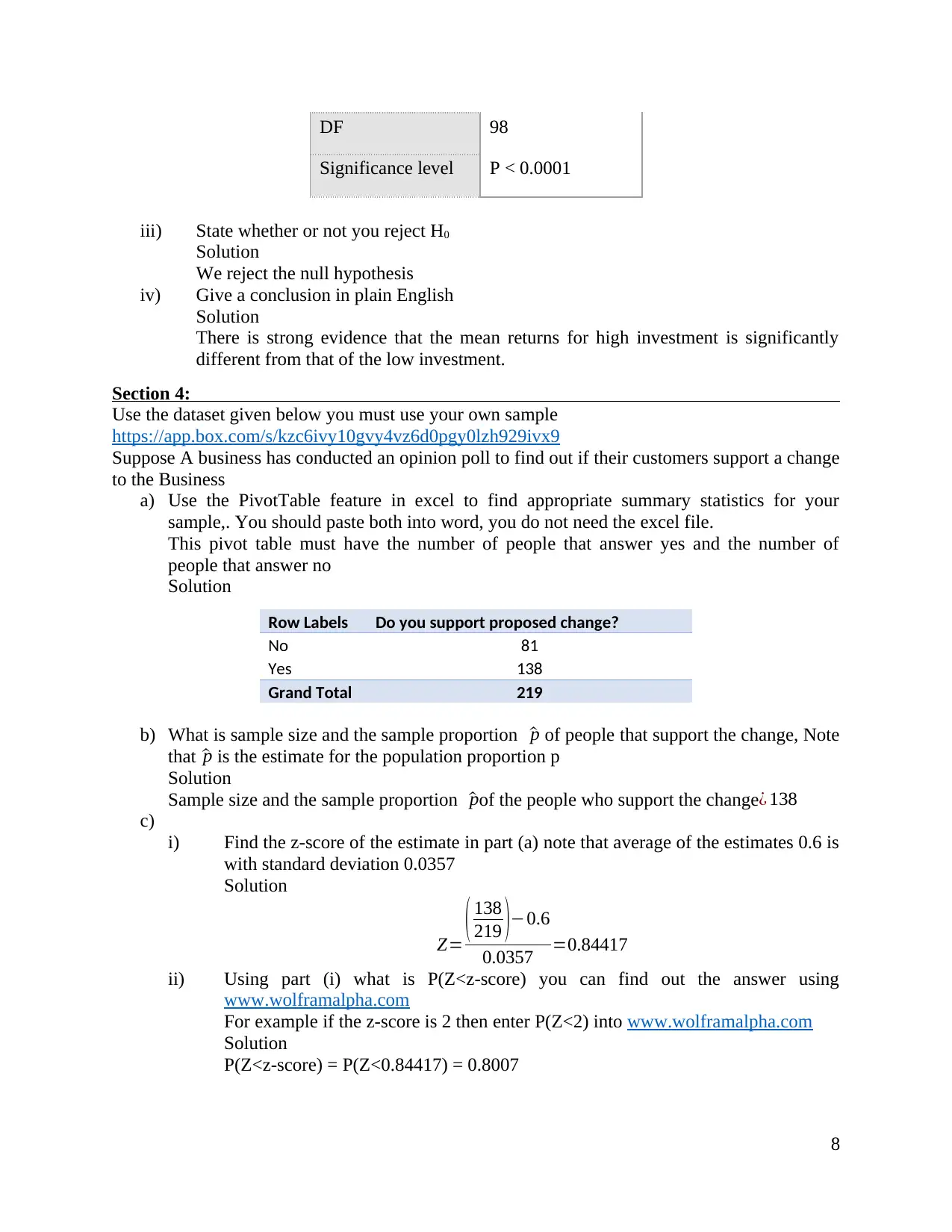
DF 98
Significance level P < 0.0001
iii) State whether or not you reject H0
Solution
We reject the null hypothesis
iv) Give a conclusion in plain English
Solution
There is strong evidence that the mean returns for high investment is significantly
different from that of the low investment.
Section 4:
Use the dataset given below you must use your own sample
https://app.box.com/s/kzc6ivy10gvy4vz6d0pgy0lzh929ivx9
Suppose A business has conducted an opinion poll to find out if their customers support a change
to the Business
a) Use the PivotTable feature in excel to find appropriate summary statistics for your
sample,. You should paste both into word, you do not need the excel file.
This pivot table must have the number of people that answer yes and the number of
people that answer no
Solution
Row Labels Do you support proposed change?
No 81
Yes 138
Grand Total 219
b) What is sample size and the sample proportion ^p of people that support the change, Note
that ^p is the estimate for the population proportion p
Solution
Sample size and the sample proportion ^pof the people who support the change¿ 138
c)
i) Find the z-score of the estimate in part (a) note that average of the estimates 0.6 is
with standard deviation 0.0357
Solution
Z= ( 138
219 )−0.6
0.0357 =0.84417
ii) Using part (i) what is P(Z<z-score) you can find out the answer using
www.wolframalpha.com
For example if the z-score is 2 then enter P(Z<2) into www.wolframalpha.com
Solution
P(Z<z-score) = P(Z<0.84417) = 0.8007
8

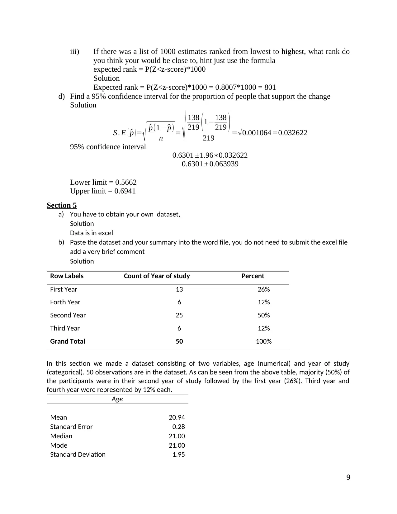
iii) If there was a list of 1000 estimates ranked from lowest to highest, what rank do
you think your would be close to, hint just use the formula
expected rank = P(Z<z-score)*1000
Solution
Expected rank = P(Z<z-score)*1000 = 0.8007*1000 = 801
d) Find a 95% confidence interval for the proportion of people that support the change
Solution
S . E ( ^p ) = √ ^p(1− ^p)
n = √ 138
219 ( 1−138
219 )
219 = √ 0.001064=0.032622
95% confidence interval
0.6301 ±1.96∗0.032622
0.6301 ± 0.063939
Lower limit = 0.5662
Upper limit = 0.6941
Section 5
a) You have to obtain your own dataset,
Solution
Data is in excel
b) Paste the dataset and your summary into the word file, you do not need to submit the excel file
add a very brief comment
Solution
Row Labels Count of Year of study Percent
First Year 13 26%
Forth Year 6 12%
Second Year 25 50%
Third Year 6 12%
Grand Total 50 100%
In this section we made a dataset consisting of two variables, age (numerical) and year of study
(categorical). 50 observations are in the dataset. As can be seen from the above table, majority (50%) of
the participants were in their second year of study followed by the first year (26%). Third year and
fourth year were represented by 12% each.
Age
Mean 20.94
Standard Error 0.28
Median 21.00
Mode 21.00
Standard Deviation 1.95
9

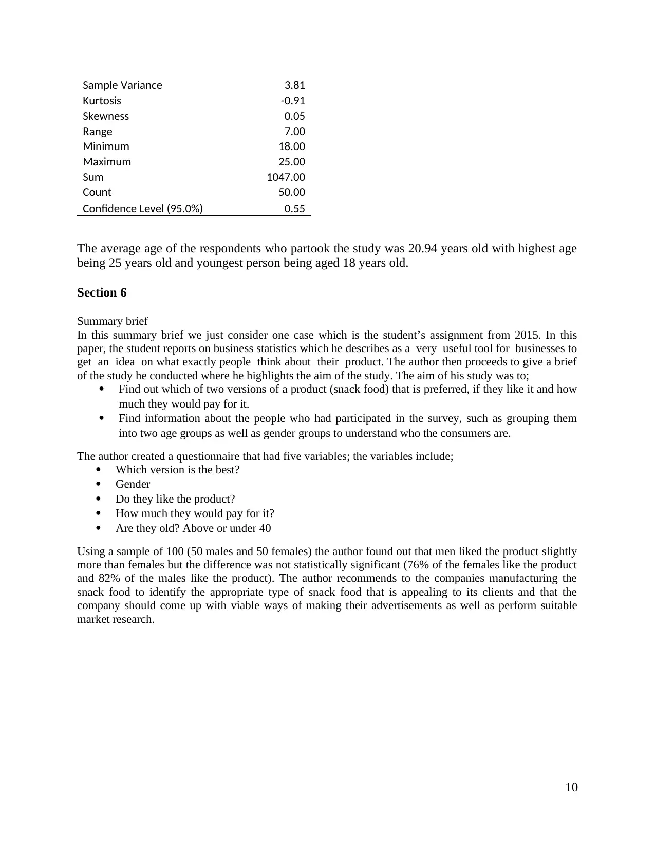
Sample Variance 3.81
Kurtosis -0.91
Skewness 0.05
Range 7.00
Minimum 18.00
Maximum 25.00
Sum 1047.00
Count 50.00
Confidence Level (95.0%) 0.55
The average age of the respondents who partook the study was 20.94 years old with highest age
being 25 years old and youngest person being aged 18 years old.
Section 6
Summary brief
In this summary brief we just consider one case which is the student’s assignment from 2015. In this
paper, the student reports on business statistics which he describes as a very useful tool for businesses to
get an idea on what exactly people think about their product. The author then proceeds to give a brief
of the study he conducted where he highlights the aim of the study. The aim of his study was to;
 Find out which of two versions of a product (snack food) that is preferred, if they like it and how
much they would pay for it.
 Find information about the people who had participated in the survey, such as grouping them
into two age groups as well as gender groups to understand who the consumers are.
The author created a questionnaire that had five variables; the variables include;
 Which version is the best?
 Gender
 Do they like the product?
 How much they would pay for it?
 Are they old? Above or under 40
Using a sample of 100 (50 males and 50 females) the author found out that men liked the product slightly
more than females but the difference was not statistically significant (76% of the females like the product
and 82% of the males like the product). The author recommends to the companies manufacturing the
snack food to identify the appropriate type of snack food that is appealing to its clients and that the
company should come up with viable ways of making their advertisements as well as perform suitable
market research.
10