Statistics for Business: Statistical Inference and Simple Regression Analysis

This article covers statistical inference and simple regression analysis for business statistics. It includes calculations, hypothesis testing, ANOVA, and testing for normal assumptions.

Running head: DATA ANALYSIS 1
Statistics for Business
Institution
Name
Id
Statistical Inference and Simple Regression Analysis

Statistics
Contents
1. Calculations Returns and Jarque- Berra Test.................................................................................3
2. Test of Hypothesis for a Single Population Mean..........................................................................4
3. The F-test: comparing equality of Variances in Two Stocks.........................................................4
4. The ANOVA Test..........................................................................................................................5
5. Excess Returns...............................................................................................................................5
6. Test of Hypothesis Using the Confidence Interval Approach........................................................7
7. Testing for normally Assumptions.................................................................................................7
References.............................................................................................................................................9
2

Statistics
1. Calculations Returns and Jarque- Berra Test
The returns for each of the stocks have been calculated using the given formula.
These returns signify the performance of the stocks (Jordan, et al., 2010). Similarly the
Jarque- Berra test of normality has been done.
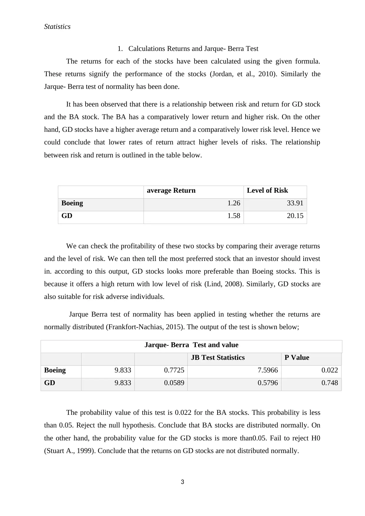
It has been observed that there is a relationship between risk and return for GD stock
and the BA stock. The BA has a comparatively lower return and higher risk. On the other
hand, GD stocks have a higher average return and a comparatively lower risk level. Hence we
could conclude that lower rates of return attract higher levels of risks. The relationship
between risk and return is outlined in the table below.
average Return Level of Risk
Boeing 1.26 33.91
GD 1.58 20.15
We can check the profitability of these two stocks by comparing their average returns
and the level of risk. We can then tell the most preferred stock that an investor should invest
in. according to this output, GD stocks looks more preferable than Boeing stocks. This is
because it offers a high return with low level of risk (Lind, 2008). Similarly, GD stocks are
also suitable for risk adverse individuals.
Jarque Berra test of normality has been applied in testing whether the returns are
normally distributed (Frankfort-Nachias, 2015). The output of the test is shown below;
Jarque- Berra Test and value
JB Test Statistics P Value
Boeing 9.833 0.7725 7.5966 0.022
GD 9.833 0.0589 0.5796 0.748
The probability value of this test is 0.022 for the BA stocks. This probability is less
than 0.05. Reject the null hypothesis. Conclude that BA stocks are distributed normally. On
the other hand, the probability value for the GD stocks is more than0.05. Fail to reject H0
(Stuart A., 1999). Conclude that the returns on GD stocks are not distributed normally.
3

Statistics
2. Test of Hypothesis for a Single Population Mean
This question aims at testing the hypothesis that the mean return of GD is not equal to
2.8 %. The sample size is sufficiently large meaning the best test is the Z test. (Frankfort-
Nachias, 2015). The hypothesis to be tested is;
H0: The mean of return on GD stocks = 2.8
H1: The mean of return on GD stocks = 2.8
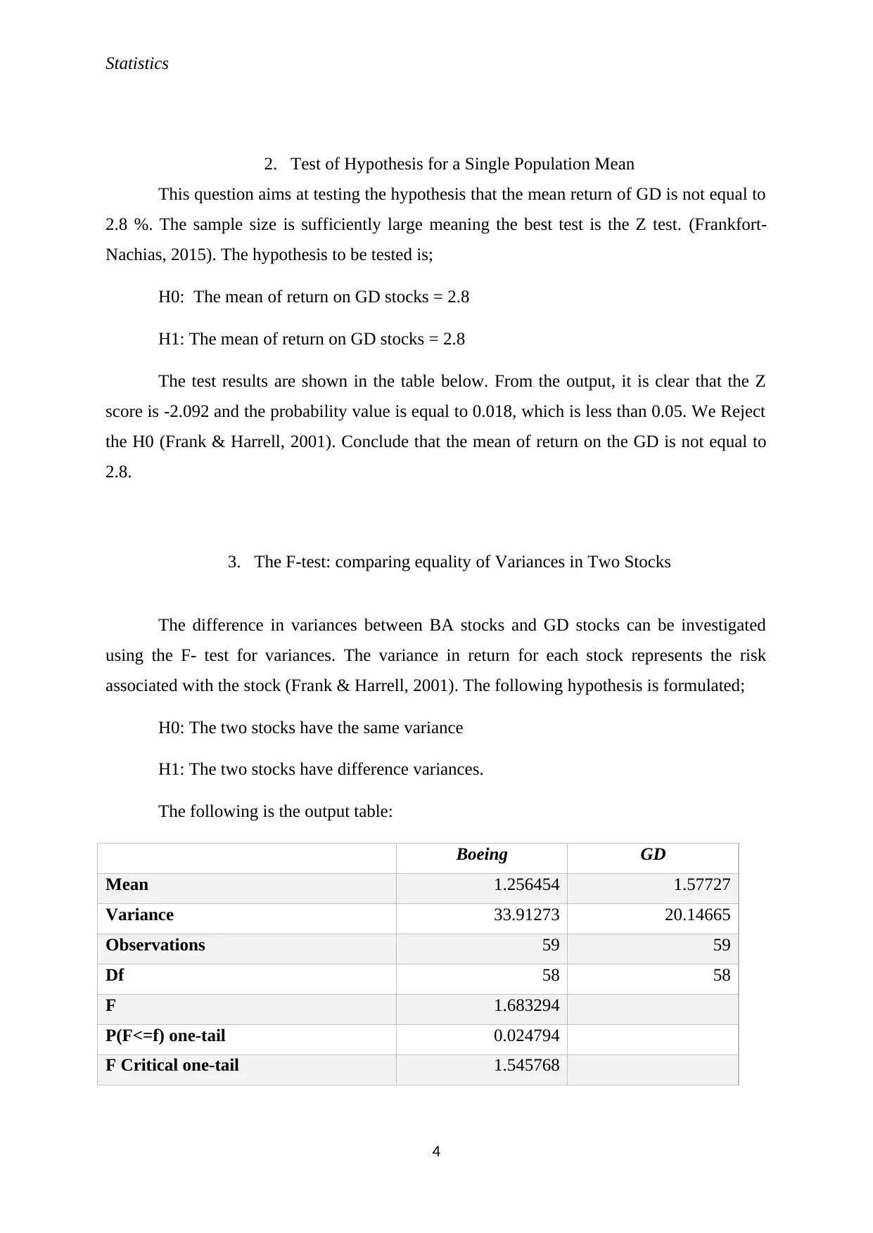
The test results are shown in the table below. From the output, it is clear that the Z
score is -2.092 and the probability value is equal to 0.018, which is less than 0.05. We Reject
the H0 (Frank & Harrell, 2001). Conclude that the mean of return on the GD is not equal to
2.8.
3. The F-test: comparing equality of Variances in Two Stocks
The difference in variances between BA stocks and GD stocks can be investigated
using the F- test for variances. The variance in return for each stock represents the risk
associated with the stock (Frank & Harrell, 2001). The following hypothesis is formulated;
H0: The two stocks have the same variance
H1: The two stocks have difference variances.
The following is the output table:
Boeing GD
Mean 1.256454 1.57727
Variance 33.91273 20.14665
Observations 59 59
Df 58 58
F 1.683294
P(F<=f) one-tail 0.024794
F Critical one-tail 1.545768
4

Statistics
The p value is 0.0024794, less than 0.05. We reject the H0. Consequently we
conclude that statistically, the returns on the two stocks are difference.
4. The ANOVA Test
Since the sample is large enough, we use the single factor ANOVA test t for equality
of means. This question is about comparison of means of two populations, Boeing and GD.
we formulate the following hypothesis;
H0: no significant difference in the average returns.
H1: There is significant difference in the average returns.
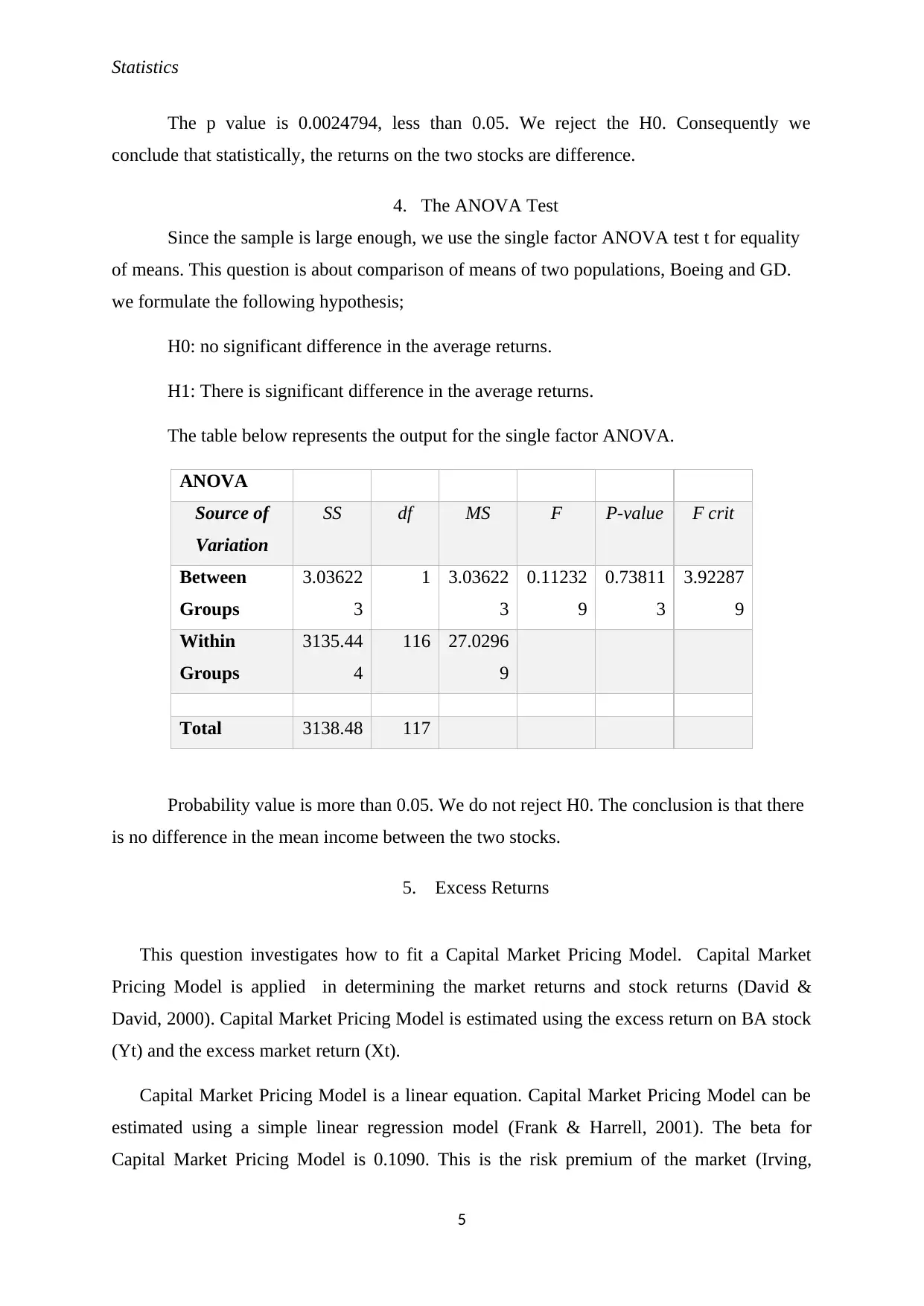
The table below represents the output for the single factor ANOVA.
ANOVA
Source of
Variation
SS df MS F P-value F crit
Between
Groups
3.03622
3
1 3.03622
3
0.11232
9
0.73811
3
3.92287
9
Within
Groups
3135.44
4
116 27.0296
9
Total 3138.48 117
Probability value is more than 0.05. We do not reject H0. The conclusion is that there
is no difference in the mean income between the two stocks.
5. Excess Returns
This question investigates how to fit a Capital Market Pricing Model. Capital Market
Pricing Model is applied in determining the market returns and stock returns (David &
David, 2000). Capital Market Pricing Model is estimated using the excess return on BA stock
(Yt) and the excess market return (Xt).
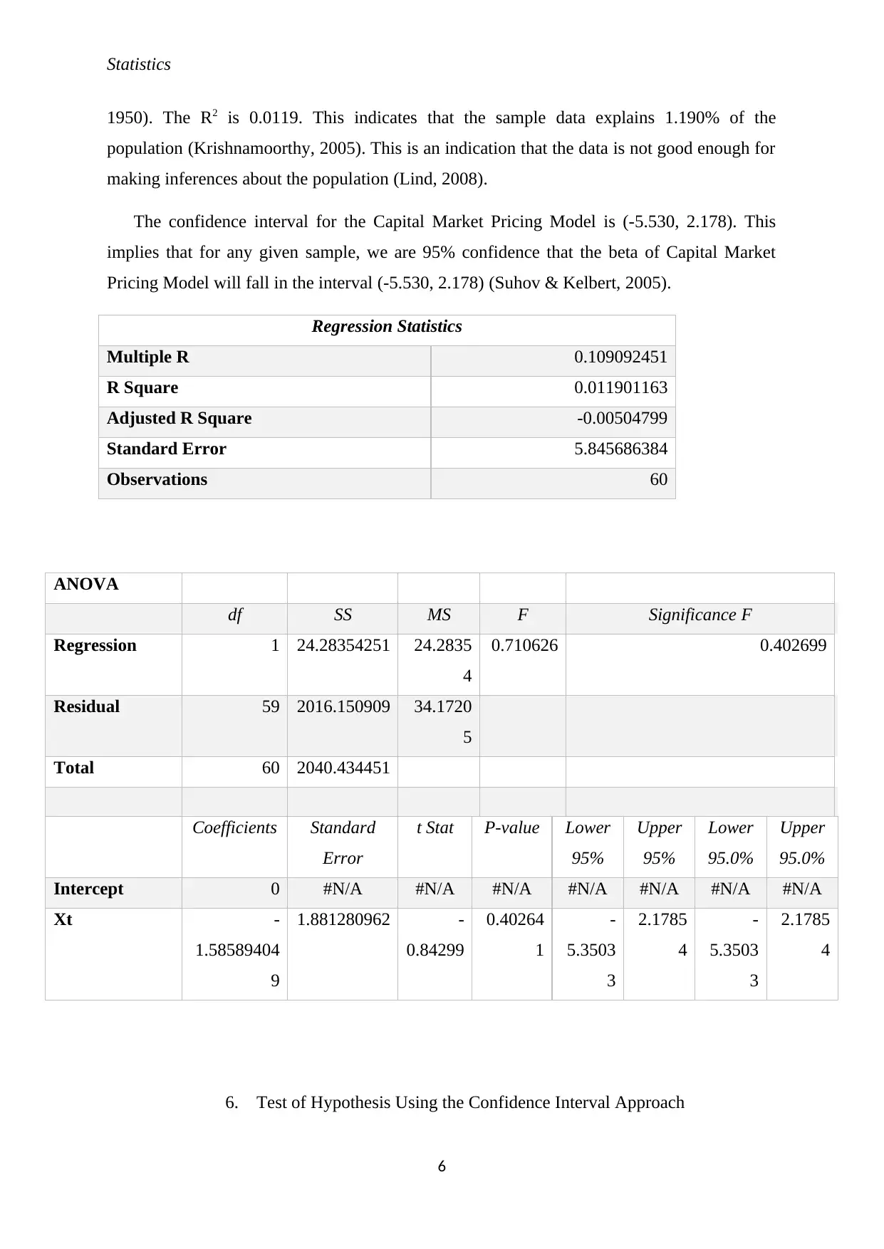
Capital Market Pricing Model is a linear equation. Capital Market Pricing Model can be
estimated using a simple linear regression model (Frank & Harrell, 2001). The beta for
Capital Market Pricing Model is 0.1090. This is the risk premium of the market (Irving,
5

Statistics
1950). The R2 is 0.0119. This indicates that the sample data explains 1.190% of the
population (Krishnamoorthy, 2005). This is an indication that the data is not good enough for
making inferences about the population (Lind, 2008).
The confidence interval for the Capital Market Pricing Model is (-5.530, 2.178). This
implies that for any given sample, we are 95% confidence that the beta of Capital Market
Pricing Model will fall in the interval (-5.530, 2.178) (Suhov & Kelbert, 2005).
ANOVA
df SS MS F Significance F
Regression 1 24.28354251 24.2835
4
0.710626 0.402699
Residual 59 2016.150909 34.1720
5
Total 60 2040.434451
Coefficients Standard
Error
t Stat P-value Lower
95%
Upper
95%
Lower
95.0%
Upper
95.0%
Intercept 0 #N/A #N/A #N/A #N/A #N/A #N/A #N/A
Xt -
1.58589404
9
1.881280962 -
0.84299
0.40264
1
-
5.3503
3
2.1785
4
-
5.3503
3
2.1785
4
6. Test of Hypothesis Using the Confidence Interval Approach
6
Regression Statistics
Multiple R 0.109092451
R Square 0.011901163
Adjusted R Square -0.00504799
Standard Error 5.845686384
Observations 60

Statistics
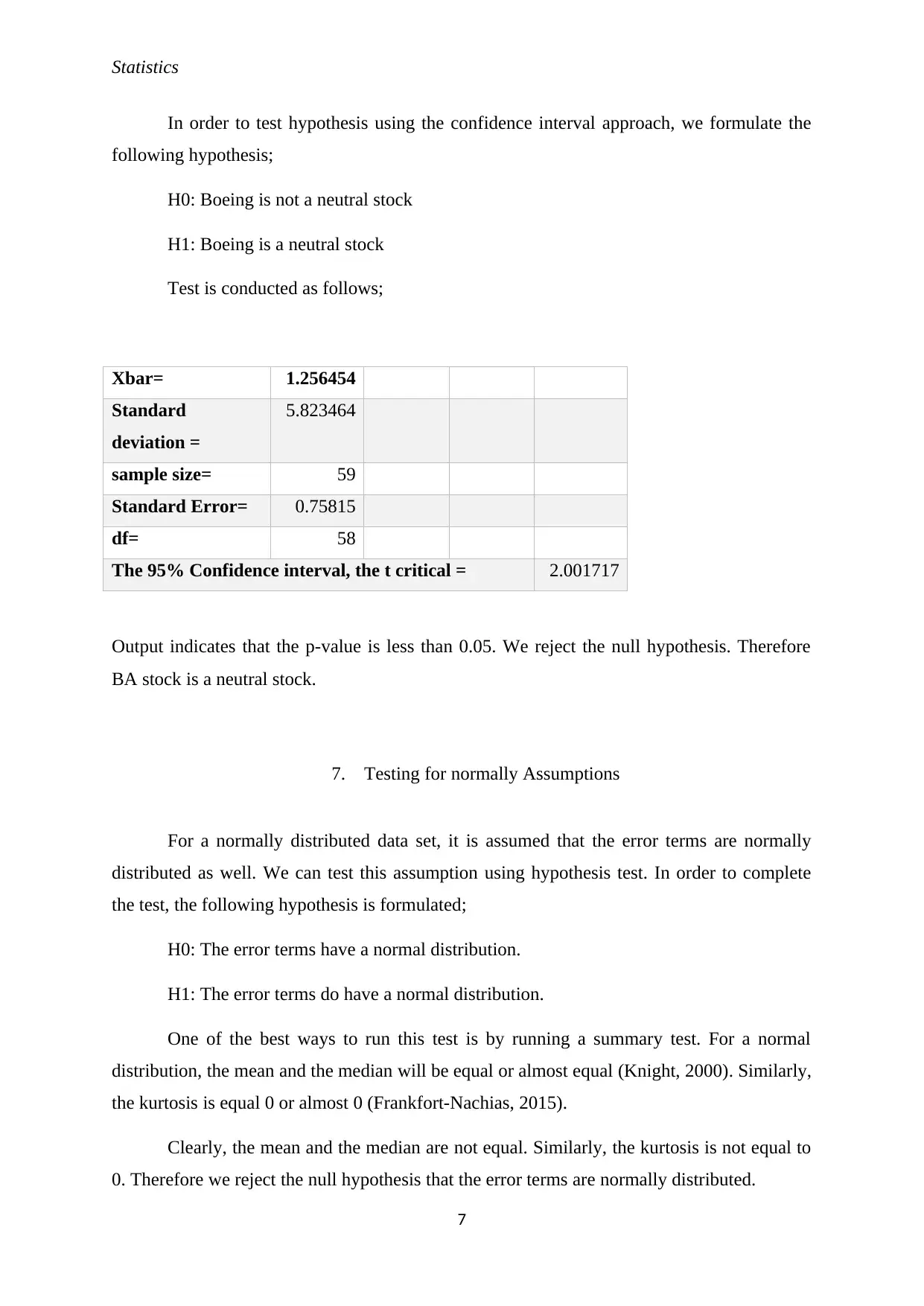
In order to test hypothesis using the confidence interval approach, we formulate the
following hypothesis;
H0: Boeing is not a neutral stock
H1: Boeing is a neutral stock
Test is conducted as follows;
Xbar= 1.256454
Standard
deviation =
5.823464
sample size= 59
Standard Error= 0.75815
df= 58
The 95% Confidence interval, the t critical = 2.001717
Output indicates that the p-value is less than 0.05. We reject the null hypothesis. Therefore
BA stock is a neutral stock.
7. Testing for normally Assumptions
For a normally distributed data set, it is assumed that the error terms are normally
distributed as well. We can test this assumption using hypothesis test. In order to complete
the test, the following hypothesis is formulated;
H0: The error terms have a normal distribution.
H1: The error terms do have a normal distribution.
One of the best ways to run this test is by running a summary test. For a normal
distribution, the mean and the median will be equal or almost equal (Knight, 2000). Similarly,
the kurtosis is equal 0 or almost 0 (Frankfort-Nachias, 2015).
Clearly, the mean and the median are not equal. Similarly, the kurtosis is not equal to
0. Therefore we reject the null hypothesis that the error terms are normally distributed.
7

Statistics
Summary Statistics
Yt Xt
Mean -0.865703331 0.007666667
Standard Error 0.750793914 0.052215674
Median -0.299915303 -0.041
Kurtosis 1.389686511 1.599
Skewness -0.598862051 0.276006434
8

Statistics
References
Ana, M., Jose, G. B. & Jorge, A. . L., 2003. Stochastic Models: Symposium on Probability and
Stochastic Processes. s.l.:s.n.
David, J. S. & David, S., 2000. Handbook of parametric and nonparametric statistical Procedures.
s.l.:s.n.
Frank, E. & Harrell, J., 2001. Regression Modelling Strategies: Models, Logistic Regression, and
Survival Analysis. s.l.:s.n.
Frankfort-Nachias, C. &. L.-G. A., 2015. Social Statistics for a diverse society. Thousand Oaks, CA: Sage
Publications.
Irving, J. G., 1950. Probability and the Weighing Evidence. s.l.:s.n.
Jordan, Stephen , A. R., Randolph, W. W. & Bradford, D., 2010. Fundamentals of corporate finance.
Boston: McGraw-Hill Irwin.
Knight, K., 2000. Mathematical Statistics- Volume in Texts in Statistical Scence Series. s.l.:Chapman
and Hall.
Krishnamoorthy, K., 2005. Handbook of Statistical Distributions with Applications. s.l.:s.n.
Lind, D. A. M. W. G. &. W. S. A., 2008. Statistical Techniques in Business &. Boston.: McGraw-Hill
Irwin.
Meigs, Walter, B. & Robert , F., 1970. Financial Accounting. s.l.:McGraw-Hill Book Company.
Sid, M., Anandi, P. S. & Robert, A. C., 2007. Practicing Financial Planning for Proffesionals.
s.l.:Rochester Hills Publishing.
Stuart A., O. K. A. S., 1999. Kendall’s Advanced Theory of Statistics: Volume 2A- Classical Inference &
the linear Model.. s.l.:s.n.
Suhov, Y. & Kelbert, M., 2005. Probability and Statisics by exasmple. basic probability and statistics.
s.l.:s.n.
Tim, S., 2005. Mastering Statistical Process Control: A handbook for Performance Improvement Using
Cases. s.l.:s.n.
9