BABS Foundation: Data Analysis and Forecasting Project Assignment
VerifiedAdded on 2022/12/27
|11
|1387
|69
Project
AI Summary
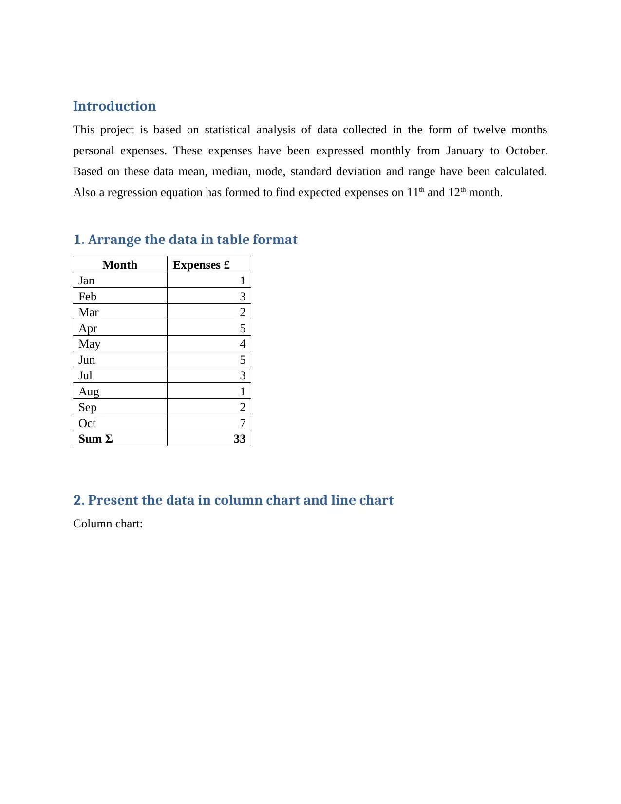
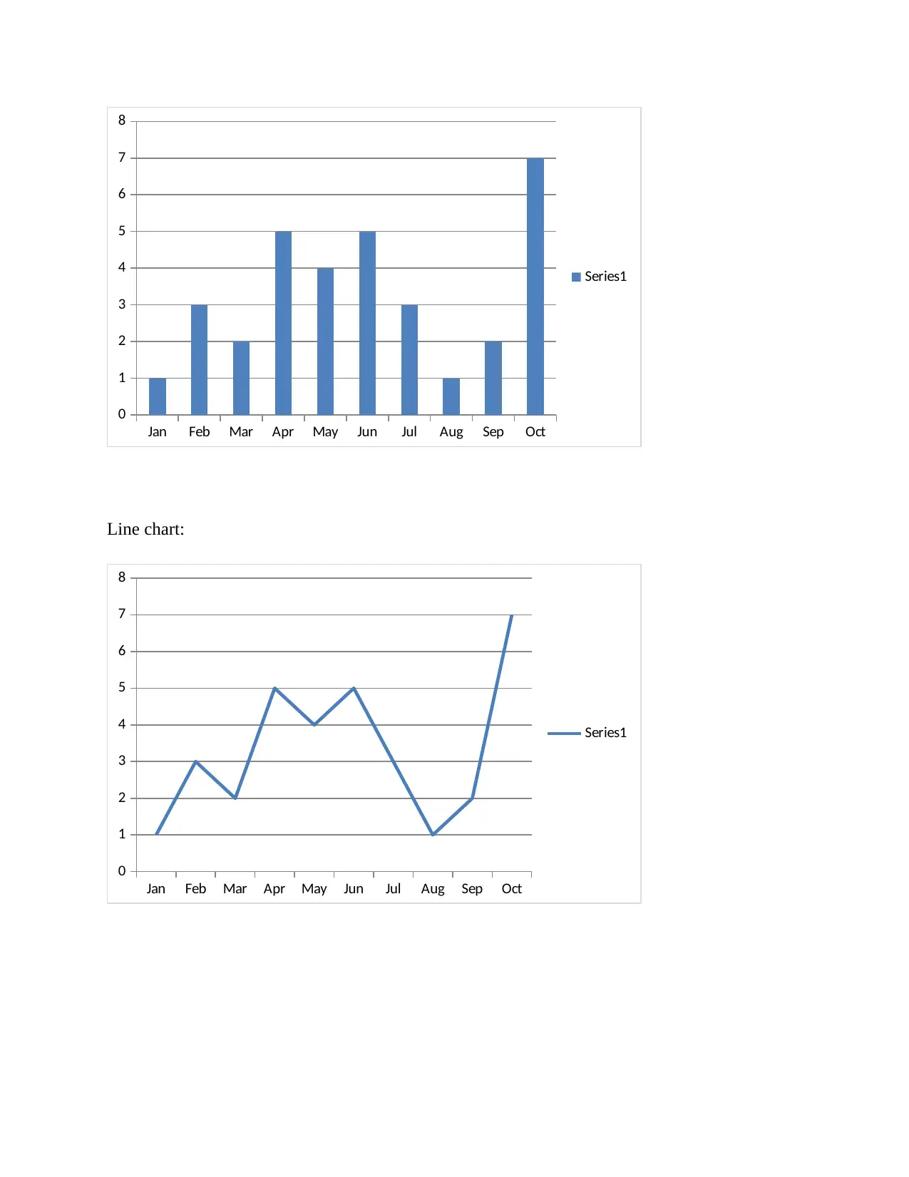
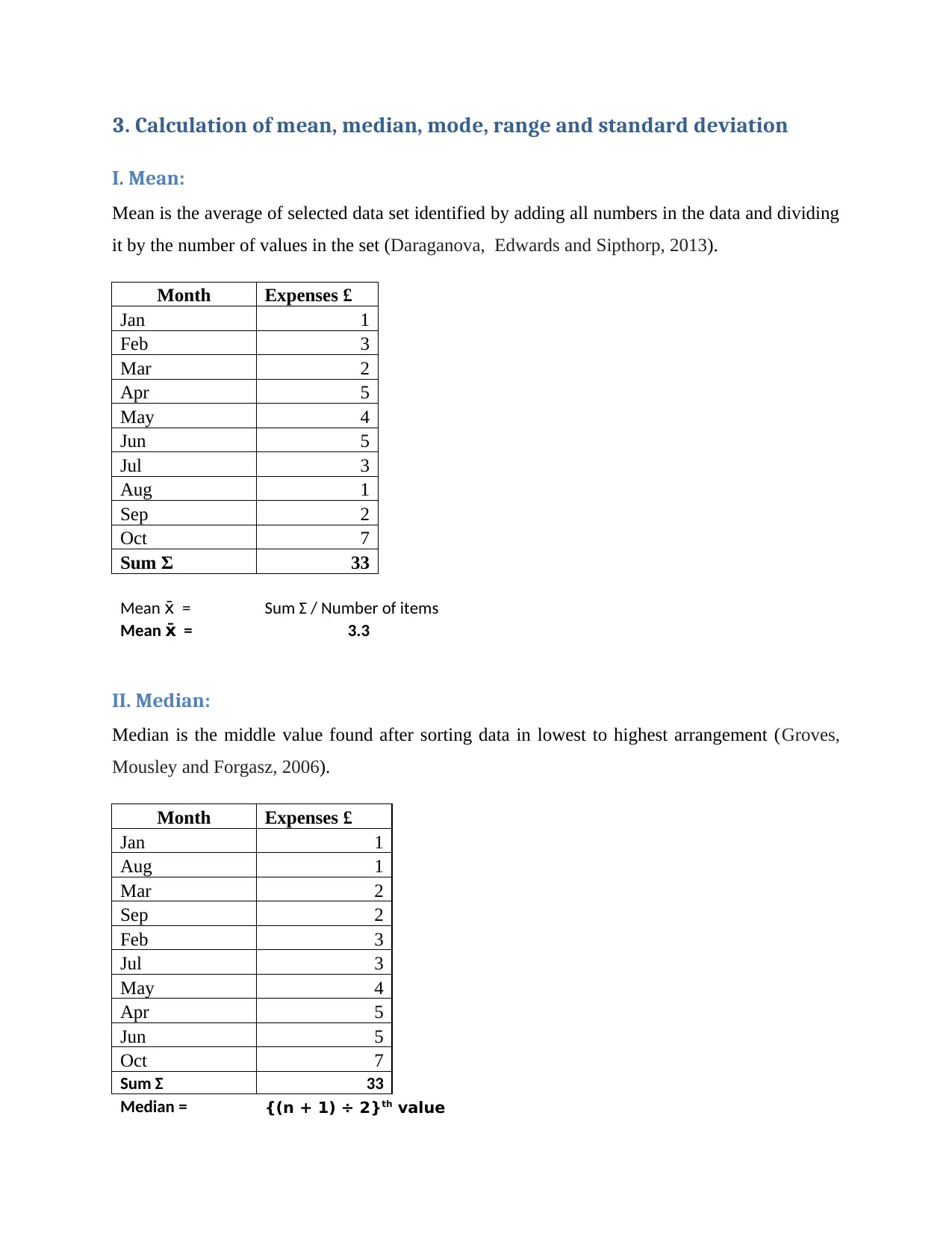
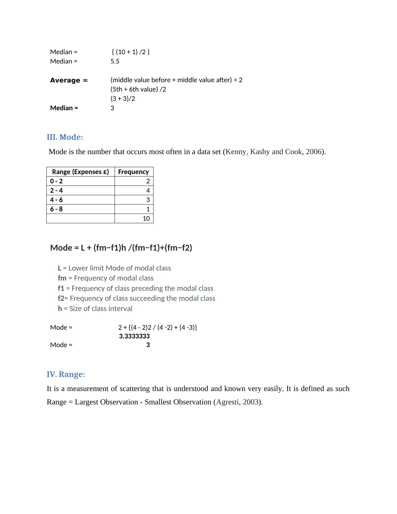
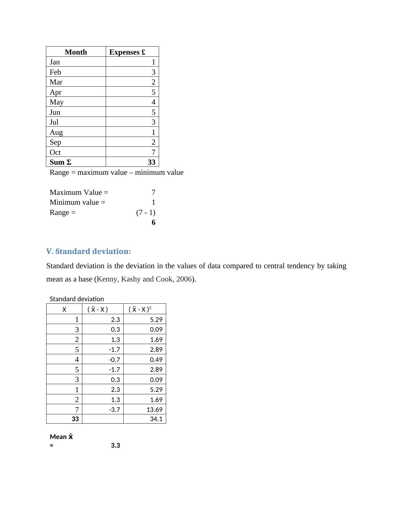
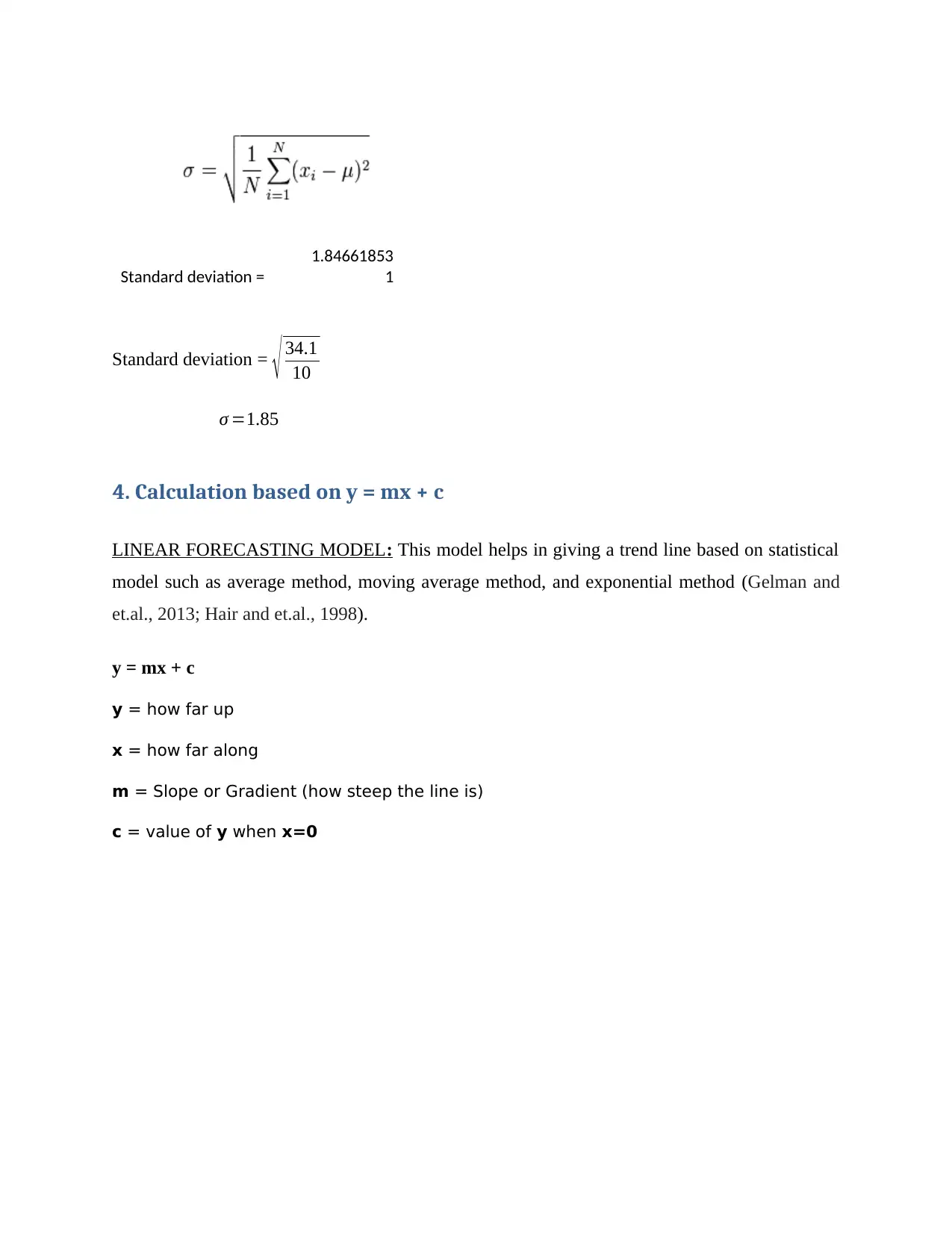
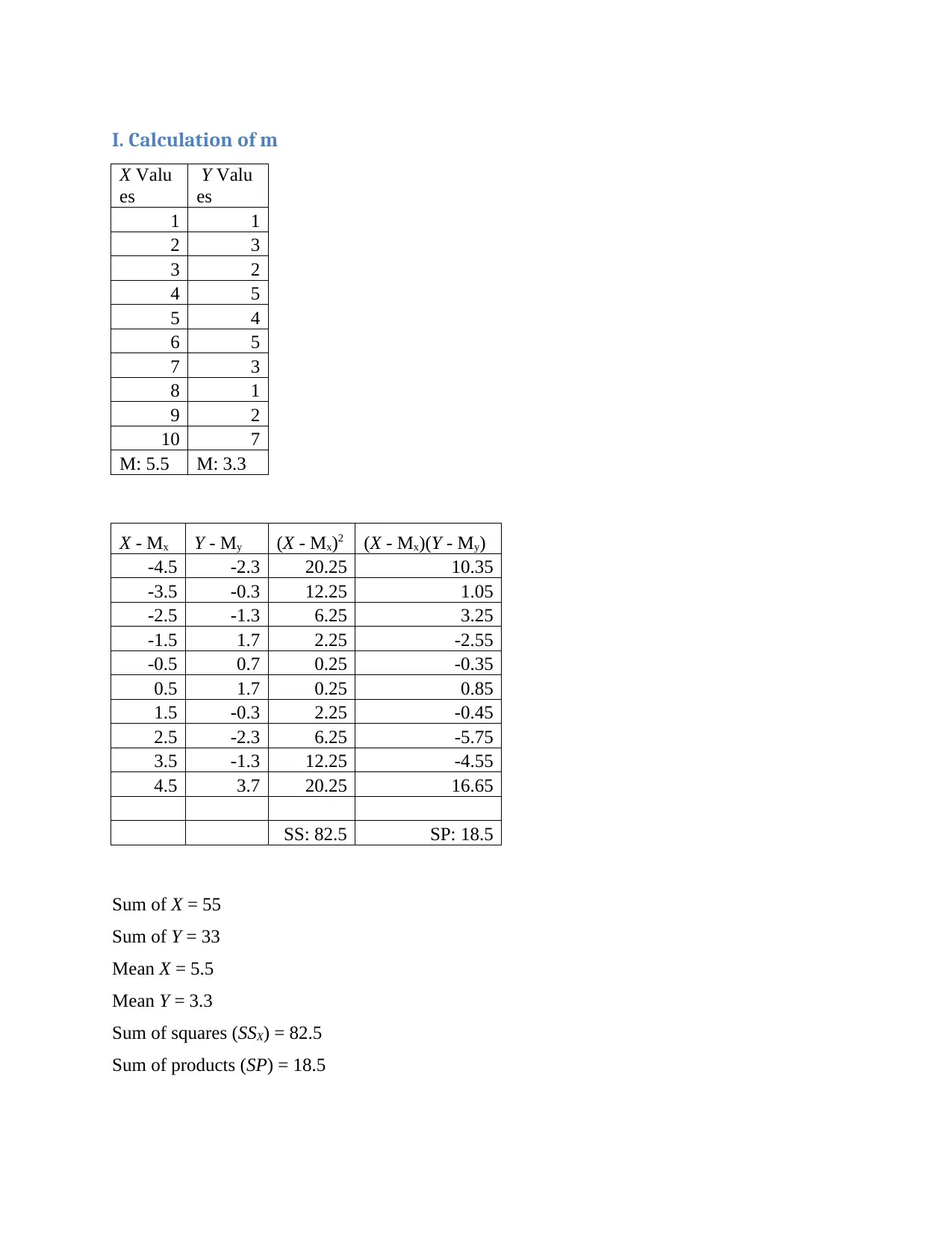
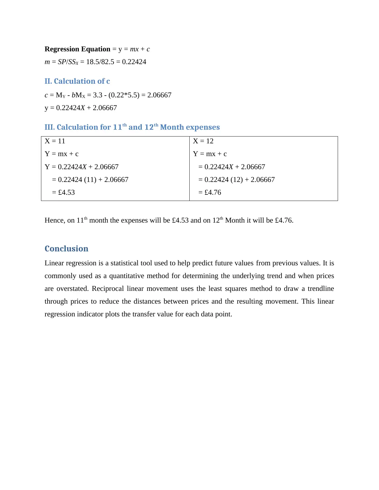
This project presents a statistical analysis of personal expenses collected over twelve months. The analysis includes arranging the data in a table format and visualizing it through column and line charts. Key statistical measures such as mean, median, mode, range, and standard deviation are calculated to understand the central tendencies and variability of the data. Furthermore, a linear regression model (y = mx + c) is developed to forecast expenses for the eleventh and twelfth months. The project concludes with a discussion on the application of linear regression as a forecasting tool, emphasizing its use in predicting future values based on historical data and highlighting its importance in identifying underlying trends. References are included to support the methodology and findings, offering a comprehensive approach to data analysis and forecasting.
1 out of 11
Related Documents


Your All-in-One AI-Powered Toolkit for Academic Success.
+13062052269
info@desklib.com
Available 24*7 on WhatsApp / Email
![[object Object]](/_next/static/media/star-bottom.7253800d.svg)
Copyright © 2020–2026 A2Z Services. All Rights Reserved. Developed and managed by ZUCOL.