Data Analysis: Correlation, Regression and Hypothesis Testing

This article discusses the analysis of data related to GPA scores of students based on gender, socio-economic status, parent education, and academic performance. It includes correlation matrix, regression models, and hypothesis testing.

Data Analysis
[1]

Task 1
1.
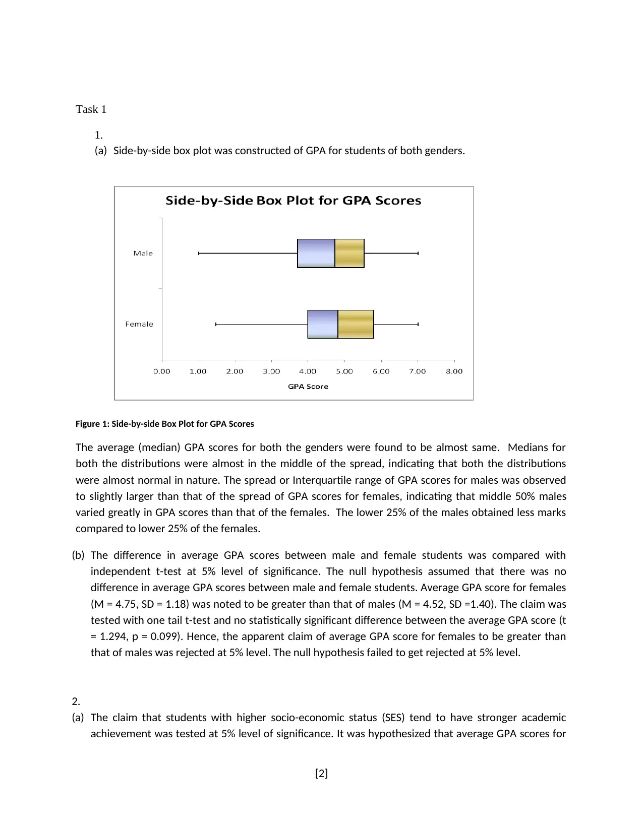
(a) Side-by-side box plot was constructed of GPA for students of both genders.
Figure 1: Side-by-side Box Plot for GPA Scores
The average (median) GPA scores for both the genders were found to be almost same. Medians for
both the distributions were almost in the middle of the spread, indicating that both the distributions
were almost normal in nature. The spread or Interquartile range of GPA scores for males was observed
to slightly larger than that of the spread of GPA scores for females, indicating that middle 50% males
varied greatly in GPA scores than that of the females. The lower 25% of the males obtained less marks
compared to lower 25% of the females.
(b) The difference in average GPA scores between male and female students was compared with
independent t-test at 5% level of significance. The null hypothesis assumed that there was no
difference in average GPA scores between male and female students. Average GPA score for females
(M = 4.75, SD = 1.18) was noted to be greater than that of males (M = 4.52, SD =1.40). The claim was
tested with one tail t-test and no statistically significant difference between the average GPA score (t
= 1.294, p = 0.099). Hence, the apparent claim of average GPA score for females to be greater than
that of males was rejected at 5% level. The null hypothesis failed to get rejected at 5% level.
2.
(a) The claim that students with higher socio-economic status (SES) tend to have stronger academic
achievement was tested at 5% level of significance. It was hypothesized that average GPA scores for
[2]

post-graduate and undergraduate were equal. The null hypothesis failed to get rejected at 5% level
as average GPA of PG_SES (M = 5.10) was found to have no statistically significant difference (t =
0.94, p = 0.176) with average GPA of UG_SES (M = 4.89). The one tail (right) test was conducted at 5%
level, and the both of the group were found to have similar GPA scores.
(b) The claim that GPA scores of students with undergraduate parents are higher (M = 4.89) than that of
the students with parents having secondary or below qualification (M = 4.08) was tested at 5% level
of significance. The null hypothesis assumed that there was no significant difference in GPA scores
between students with parents as undergraduate and secondary level. The null hypothesis was
rejected (t = - 4.291, p < 0.05) at 5% level, indicating that GPA scores of students with undergraduate
parents are significantly higher than that of the students with parents having secondary or below
qualification.
Task 2
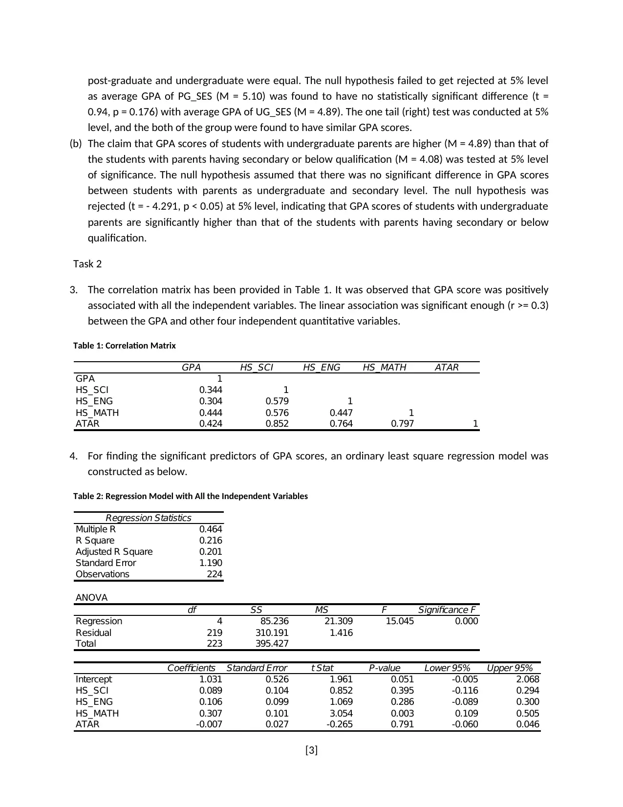
3. The correlation matrix has been provided in Table 1. It was observed that GPA score was positively
associated with all the independent variables. The linear association was significant enough (r >= 0.3)
between the GPA and other four independent quantitative variables.
Table 1: Correlation Matrix
GPA HS_SCI HS_ENG HS_MATH ATAR
GPA 1
HS_SCI 0.344 1
HS_ENG 0.304 0.579 1
HS_MATH 0.444 0.576 0.447 1
ATAR 0.424 0.852 0.764 0.797 1
4. For finding the significant predictors of GPA scores, an ordinary least square regression model was
constructed as below.
Table 2: Regression Model with All the Independent Variables
Regression Statistics
Multiple R 0.464
R Square 0.216
Adjusted R Square 0.201
Standard Error 1.190
Observations 224
ANOVA
df SS MS F Significance F
Regression 4 85.236 21.309 15.045 0.000
Residual 219 310.191 1.416
Total 223 395.427
Coefficients Standard Error t Stat P-value Lower 95% Upper 95%
Intercept 1.031 0.526 1.961 0.051 -0.005 2.068
HS_SCI 0.089 0.104 0.852 0.395 -0.116 0.294
HS_ENG 0.106 0.099 1.069 0.286 -0.089 0.300
HS_MATH 0.307 0.101 3.054 0.003 0.109 0.505
ATAR -0.007 0.027 -0.265 0.791 -0.060 0.046
[3]

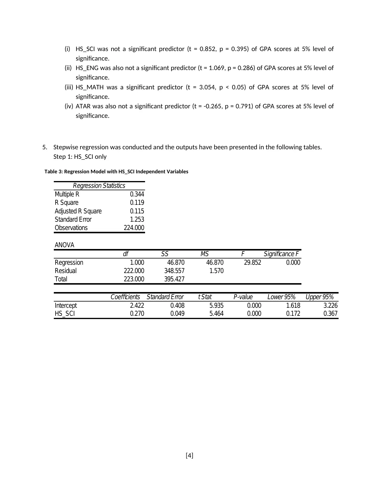
(i) HS_SCI was not a significant predictor (t = 0.852, p = 0.395) of GPA scores at 5% level of
significance.
(ii) HS_ENG was also not a significant predictor (t = 1.069, p = 0.286) of GPA scores at 5% level of
significance.
(iii) HS_MATH was a significant predictor (t = 3.054, p < 0.05) of GPA scores at 5% level of
significance.
(iv) ATAR was also not a significant predictor (t = -0.265, p = 0.791) of GPA scores at 5% level of
significance.
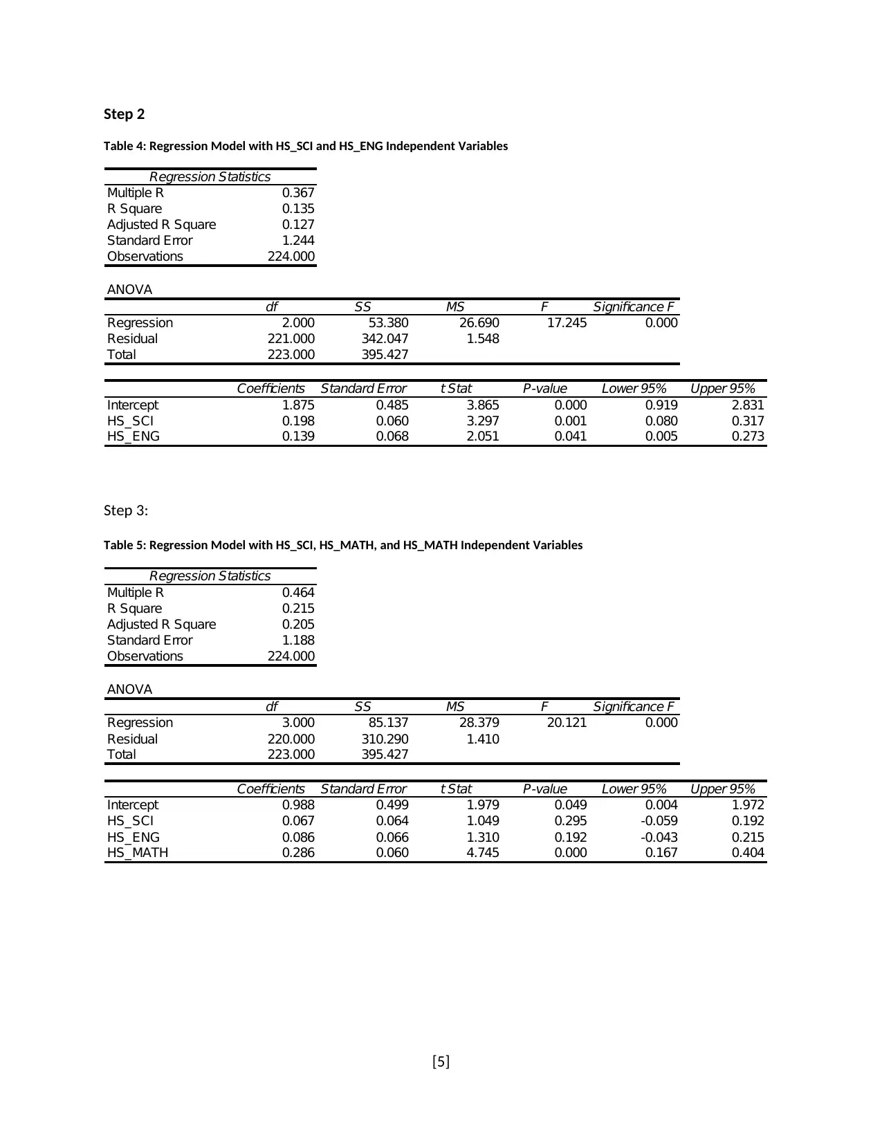
5. Stepwise regression was conducted and the outputs have been presented in the following tables.
Step 1: HS_SCI only
Table 3: Regression Model with HS_SCI Independent Variables
Regression Statistics
Multiple R 0.344
R Square 0.119
Adjusted R Square 0.115
Standard Error 1.253
Observations 224.000
ANOVA
df SS MS F Significance F
Regression 1.000 46.870 46.870 29.852 0.000
Residual 222.000 348.557 1.570
Total 223.000 395.427
Coefficients Standard Error t Stat P-value Lower 95% Upper 95%
Intercept 2.422 0.408 5.935 0.000 1.618 3.226
HS_SCI 0.270 0.049 5.464 0.000 0.172 0.367
[4]

Step 2
Table 4: Regression Model with HS_SCI and HS_ENG Independent Variables
Regression Statistics
Multiple R 0.367
R Square 0.135
Adjusted R Square 0.127
Standard Error 1.244
Observations 224.000
ANOVA
df SS MS F Significance F
Regression 2.000 53.380 26.690 17.245 0.000
Residual 221.000 342.047 1.548
Total 223.000 395.427
Coefficients Standard Error t Stat P-value Lower 95% Upper 95%
Intercept 1.875 0.485 3.865 0.000 0.919 2.831
HS_SCI 0.198 0.060 3.297 0.001 0.080 0.317
HS_ENG 0.139 0.068 2.051 0.041 0.005 0.273
Step 3:
Table 5: Regression Model with HS_SCI, HS_MATH, and HS_MATH Independent Variables
Regression Statistics
Multiple R 0.464
R Square 0.215
Adjusted R Square 0.205
Standard Error 1.188
Observations 224.000
ANOVA
df SS MS F Significance F
Regression 3.000 85.137 28.379 20.121 0.000
Residual 220.000 310.290 1.410
Total 223.000 395.427
Coefficients Standard Error t Stat P-value Lower 95% Upper 95%
Intercept 0.988 0.499 1.979 0.049 0.004 1.972
HS_SCI 0.067 0.064 1.049 0.295 -0.059 0.192
HS_ENG 0.086 0.066 1.310 0.192 -0.043 0.215
HS_MATH 0.286 0.060 4.745 0.000 0.167 0.404
[5]

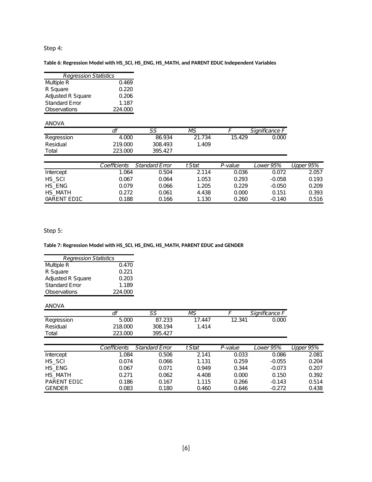
Step 4:
Table 6: Regression Model with HS_SCI, HS_ENG, HS_MATH, and PARENT EDUC Independent Variables
Regression Statistics
Multiple R 0.469
R Square 0.220
Adjusted R Square 0.206
Standard Error 1.187
Observations 224.000
ANOVA
df SS MS F Significance F
Regression 4.000 86.934 21.734 15.429 0.000
Residual 219.000 308.493 1.409
Total 223.000 395.427
Coefficients Standard Error t Stat P-value Lower 95% Upper 95%
Intercept 1.064 0.504 2.114 0.036 0.072 2.057
HS_SCI 0.067 0.064 1.053 0.293 -0.058 0.193
HS_ENG 0.079 0.066 1.205 0.229 -0.050 0.209
HS_MATH 0.272 0.061 4.438 0.000 0.151 0.393
0ARENT ED1C 0.188 0.166 1.130 0.260 -0.140 0.516
Step 5:
Table 7: Regression Model with HS_SCI, HS_ENG, HS_MATH, PARENT EDUC and GENDER
Regression Statistics
Multiple R 0.470
R Square 0.221
Adjusted R Square 0.203
Standard Error 1.189
Observations 224.000
ANOVA
df SS MS F Significance F
Regression 5.000 87.233 17.447 12.341 0.000
Residual 218.000 308.194 1.414
Total 223.000 395.427
Coefficients Standard Error t Stat P-value Lower 95% Upper 95%
Intercept 1.084 0.506 2.141 0.033 0.086 2.081
HS_SCI 0.074 0.066 1.131 0.259 -0.055 0.204
HS_ENG 0.067 0.071 0.949 0.344 -0.073 0.207
HS_MATH 0.271 0.062 4.408 0.000 0.150 0.392
PARENT ED1C 0.186 0.167 1.115 0.266 -0.143 0.514
GENDER 0.083 0.180 0.460 0.646 -0.272 0.438
[6]

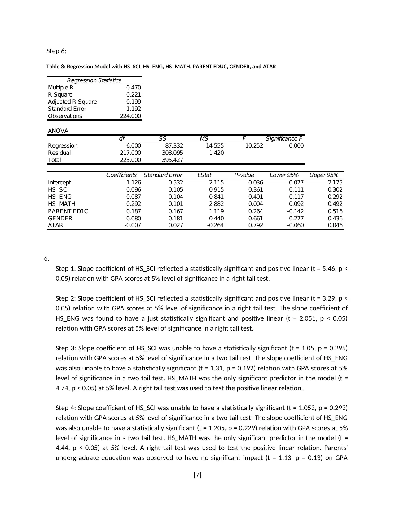
Step 6:
Table 8: Regression Model with HS_SCI, HS_ENG, HS_MATH, PARENT EDUC, GENDER, and ATAR
Regression Statistics
Multiple R 0.470
R Square 0.221
Adjusted R Square 0.199
Standard Error 1.192
Observations 224.000
ANOVA
df SS MS F Significance F
Regression 6.000 87.332 14.555 10.252 0.000
Residual 217.000 308.095 1.420
Total 223.000 395.427
Coefficients Standard Error t Stat P-value Lower 95% Upper 95%
Intercept 1.126 0.532 2.115 0.036 0.077 2.175
HS_SCI 0.096 0.105 0.915 0.361 -0.111 0.302
HS_ENG 0.087 0.104 0.841 0.401 -0.117 0.292
HS_MATH 0.292 0.101 2.882 0.004 0.092 0.492
PARENT ED1C 0.187 0.167 1.119 0.264 -0.142 0.516
GENDER 0.080 0.181 0.440 0.661 -0.277 0.436
ATAR -0.007 0.027 -0.264 0.792 -0.060 0.046
6.
Step 1: Slope coefficient of HS_SCI reflected a statistically significant and positive linear (t = 5.46, p <
0.05) relation with GPA scores at 5% level of significance in a right tail test.
Step 2: Slope coefficient of HS_SCI reflected a statistically significant and positive linear (t = 3.29, p <
0.05) relation with GPA scores at 5% level of significance in a right tail test. The slope coefficient of
HS_ENG was found to have a just statistically significant and positive linear (t = 2.051, p < 0.05)
relation with GPA scores at 5% level of significance in a right tail test.
Step 3: Slope coefficient of HS_SCI was unable to have a statistically significant (t = 1.05, p = 0.295)
relation with GPA scores at 5% level of significance in a two tail test. The slope coefficient of HS_ENG
was also unable to have a statistically significant (t = 1.31, p = 0.192) relation with GPA scores at 5%
level of significance in a two tail test. HS_MATH was the only significant predictor in the model (t =
4.74, p < 0.05) at 5% level. A right tail test was used to test the positive linear relation.
Step 4: Slope coefficient of HS_SCI was unable to have a statistically significant (t = 1.053, p = 0.293)
relation with GPA scores at 5% level of significance in a two tail test. The slope coefficient of HS_ENG
was also unable to have a statistically significant (t = 1.205, p = 0.229) relation with GPA scores at 5%
level of significance in a two tail test. HS_MATH was the only significant predictor in the model (t =
4.44, p < 0.05) at 5% level. A right tail test was used to test the positive linear relation. Parents’
undergraduate education was observed to have no significant impact (t = 1.13, p = 0.13) on GPA
[7]

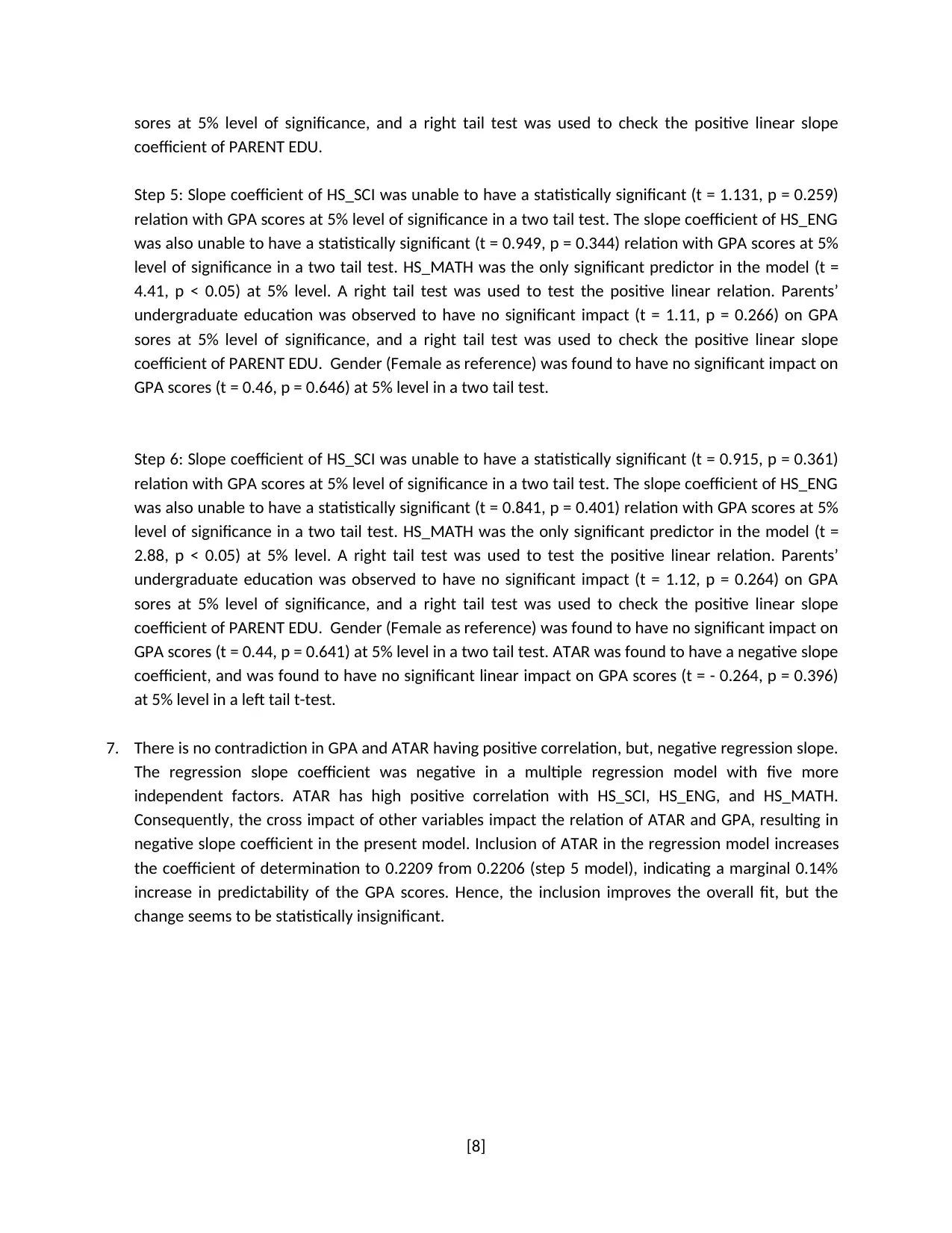
sores at 5% level of significance, and a right tail test was used to check the positive linear slope
coefficient of PARENT EDU.
Step 5: Slope coefficient of HS_SCI was unable to have a statistically significant (t = 1.131, p = 0.259)
relation with GPA scores at 5% level of significance in a two tail test. The slope coefficient of HS_ENG
was also unable to have a statistically significant (t = 0.949, p = 0.344) relation with GPA scores at 5%
level of significance in a two tail test. HS_MATH was the only significant predictor in the model (t =
4.41, p < 0.05) at 5% level. A right tail test was used to test the positive linear relation. Parents’
undergraduate education was observed to have no significant impact (t = 1.11, p = 0.266) on GPA
sores at 5% level of significance, and a right tail test was used to check the positive linear slope
coefficient of PARENT EDU. Gender (Female as reference) was found to have no significant impact on
GPA scores (t = 0.46, p = 0.646) at 5% level in a two tail test.
Step 6: Slope coefficient of HS_SCI was unable to have a statistically significant (t = 0.915, p = 0.361)
relation with GPA scores at 5% level of significance in a two tail test. The slope coefficient of HS_ENG
was also unable to have a statistically significant (t = 0.841, p = 0.401) relation with GPA scores at 5%
level of significance in a two tail test. HS_MATH was the only significant predictor in the model (t =
2.88, p < 0.05) at 5% level. A right tail test was used to test the positive linear relation. Parents’
undergraduate education was observed to have no significant impact (t = 1.12, p = 0.264) on GPA
sores at 5% level of significance, and a right tail test was used to check the positive linear slope
coefficient of PARENT EDU. Gender (Female as reference) was found to have no significant impact on
GPA scores (t = 0.44, p = 0.641) at 5% level in a two tail test. ATAR was found to have a negative slope
coefficient, and was found to have no significant linear impact on GPA scores (t = - 0.264, p = 0.396)
at 5% level in a left tail t-test.
7. There is no contradiction in GPA and ATAR having positive correlation, but, negative regression slope.
The regression slope coefficient was negative in a multiple regression model with five more
independent factors. ATAR has high positive correlation with HS_SCI, HS_ENG, and HS_MATH.
Consequently, the cross impact of other variables impact the relation of ATAR and GPA, resulting in
negative slope coefficient in the present model. Inclusion of ATAR in the regression model increases
the coefficient of determination to 0.2209 from 0.2206 (step 5 model), indicating a marginal 0.14%
increase in predictability of the GPA scores. Hence, the inclusion improves the overall fit, but the
change seems to be statistically insignificant.
[8]

Task 3
Summary Report
The GPA scores of the students were found to have impact of the educational background (students’
social economic status). But, no significant difference in average GPA scores was noted for parents’
postgraduate education as compared to undergraduate education. However, parents with secondary or
lower education was observed to have a negative impact on GPA scores, and the comparison with GPA
scores of students with undergraduate parents yielded a statistically significant difference (t = - 4.29, p <
0.05). Gender of the students was not a significantly decisive factor for higher GPA scores (t = 1.294, p =
0.197), and average GPA scores were almost same for the two genders. GPA scores were correlated with
the independent impact factors in a positive direction. HS_SCI was noted to be a statistically significant
predictor of GPA scores in a simple regression (t = 5.46, p < 0.05), and significant predictor (t = 3.29, p <
0.05) as well with HS_ENG as a predictor in a multiple regression model. Inclusion of HS_MATH made
HS_SCI an insignificant impact factor (t = 1.05, p = 0.295), probably due to the huge statistical impact of
Math on GPA scores. It was possible to conclude that students with higher marks of mathematics were
significantly oriented towards the science courses. Hence, marks in science was a good predictor, but was
suppressed by impact of mathematics scores. Australian Tertiary Admission Rank was observed to have
positive significant correlation with GPA scores, and had high positive correlation with scores in other
three subjects. But, in the Multiple Regression Model, due to strong presence of Mathematics,
significance of ATAR scores was insignificant. Hence, inclusion was ATAR was an option but not an
essentiality. The best regression model would be the model in step 3 with HS_SCI, HS_ENG, and
HS_MATH as predictors. The model would be able to explain 21.5% variation in GPA and adjusted R-
square due to inclusion of the independent factors would change by only 5%, to 20.5%. ATAR, PARENT
EDU, and gender were excluded from the model. These variables have insignificant impact on the GPA
scores of the students, especially in presence of mathematics as a predictor.
[9]