Decision Support Tools and Statistics Problems

The assignment provided covers various aspects of decision support tools and statistics, including discrete and continuous probability distributions, sample space and probability calculations, statistical tests for mean time and standard deviation, and a one-sample t-test. The problems are based on real-world scenarios such as average sales of loaves of bread, daily sales of apples, and the population and sex distribution of Australia in 2017. The document is suitable for students looking for past papers and solved assignments on decision support tools and statistics.

Running Head: DECISION SUPPORT TOOLS
Decision Support Tools
Name of the Student
Name of the University
Author Note

1DECISION SUPPORT TOOLS
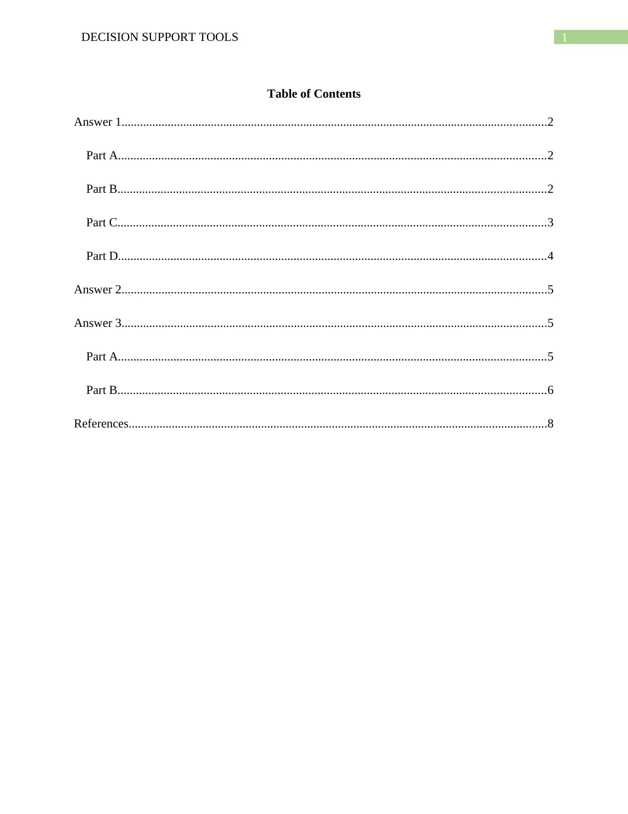
Table of Contents
Answer 1..........................................................................................................................................2
Part A...........................................................................................................................................2
Part B...........................................................................................................................................2
Part C...........................................................................................................................................3
Part D...........................................................................................................................................4
Answer 2..........................................................................................................................................5
Answer 3..........................................................................................................................................5
Part A...........................................................................................................................................5
Part B...........................................................................................................................................6
References........................................................................................................................................8

2DECISION SUPPORT TOOLS
Answer 1
Part A
A statement of all possible values or sets of values of a random variable together with the
corresponding probabilities gives the probability distribution of the random variable. It may be
represented by a function, in a table or a graph (Rohatgi & Saleh, 2015).
The probability distribution of a discrete random variable is known as a discrete
probability distribution. In a discrete probability distribution, the probabilities of the random
variables at each of the discrete points must be greater than zero and sum of all the probabilities
are equal to 1 (Rohatgi & Saleh, 2015). For example, if a die is rolled and a six is obtained, then
the person gets a gift. If a six is not obtained, no gift is given. This is an example of a discrete
probability distribution where the probability of obtaining a six is 1
6 and not obtaining a six is 5
6 .
The probability distribution of a continuous random variable is known as continuous
probability distribution. In continuous probability distribution, there are no distinct points at
which the probabilities can be checked and hence the probabilities at each point is considered as
zero. The area under the curve of the probability distribution function over its whole range of
values is equal to 1 (Rohatgi & Saleh, 2015). For example, there is a guessing game where if a
person can guess the price of the product within $2 of the original price, the person gets a gift,
otherwise not. This is an example of a continuous probability distribution.
Part B
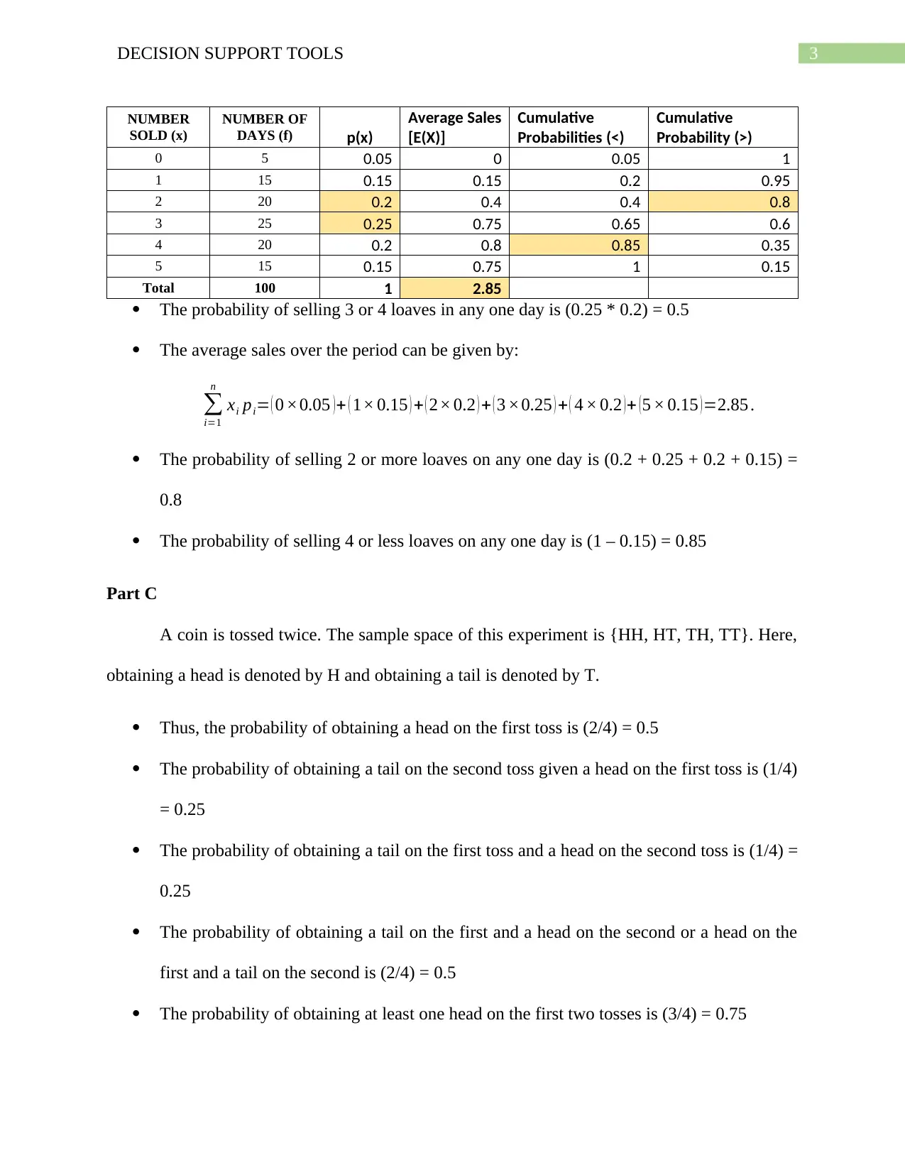
The daily sales of the top selling loaf of bread of a baker, over the last 100 days is given
in the following table:

3DECISION SUPPORT TOOLS
NUMBER
SOLD (x)
NUMBER OF
DAYS (f) p(x)
Average Sales
[E(X)]
Cumulative
Probabilities (<)
Cumulative
Probability (>)
0 5 0.05 0 0.05 1
1 15 0.15 0.15 0.2 0.95
2 20 0.2 0.4 0.4 0.8
3 25 0.25 0.75 0.65 0.6
4 20 0.2 0.8 0.85 0.35
5 15 0.15 0.75 1 0.15
Total 100 1 2.85
 The probability of selling 3 or 4 loaves in any one day is (0.25 * 0.2) = 0.5
 The average sales over the period can be given by:
∑
i=1
n
xi pi= ( 0 ×0.05 )+ ( 1× 0.15 ) + ( 2× 0.2 ) + ( 3 ×0.25 ) + ( 4 × 0.2 )+ (5 × 0.15 )=2.85 .
 The probability of selling 2 or more loaves on any one day is (0.2 + 0.25 + 0.2 + 0.15) =
0.8
 The probability of selling 4 or less loaves on any one day is (1 – 0.15) = 0.85
Part C
A coin is tossed twice. The sample space of this experiment is {HH, HT, TH, TT}. Here,
obtaining a head is denoted by H and obtaining a tail is denoted by T.
 Thus, the probability of obtaining a head on the first toss is (2/4) = 0.5
 The probability of obtaining a tail on the second toss given a head on the first toss is (1/4)
= 0.25
 The probability of obtaining a tail on the first toss and a head on the second toss is (1/4) =
0.25
 The probability of obtaining a tail on the first and a head on the second or a head on the
first and a tail on the second is (2/4) = 0.5
 The probability of obtaining at least one head on the first two tosses is (3/4) = 0.75

4DECISION SUPPORT TOOLS
Part D
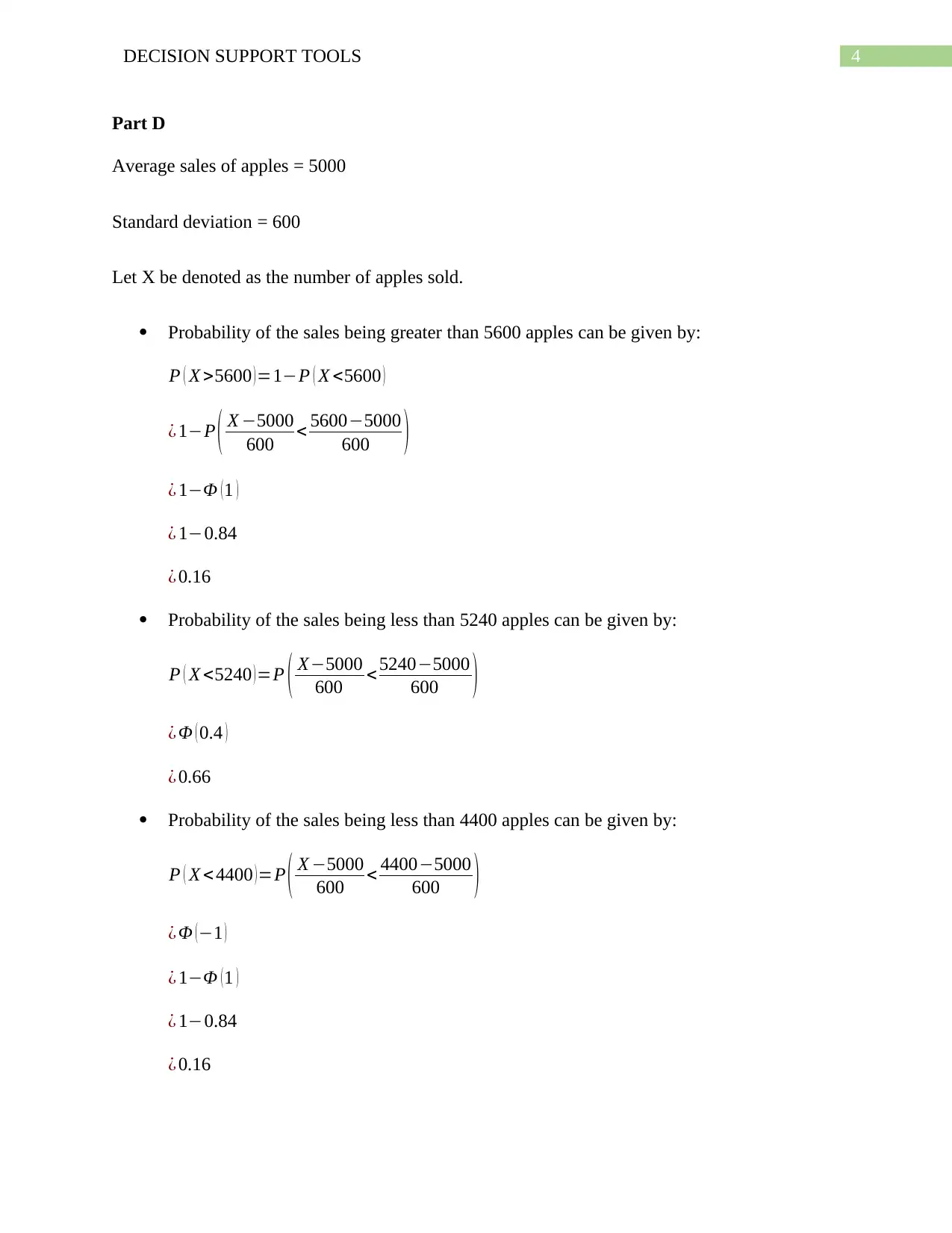
Average sales of apples = 5000
Standard deviation = 600
Let X be denoted as the number of apples sold.
 Probability of the sales being greater than 5600 apples can be given by:
P ( X >5600 )=1−P ( X <5600 )
¿ 1−P ( X −5000
600 < 5600−5000
600 )
¿ 1−Φ ( 1 )
¿ 1−0.84
¿ 0.16
 Probability of the sales being less than 5240 apples can be given by:
P ( X <5240 )=P ( X−5000
600 < 5240−5000
600 )
¿ Φ ( 0.4 )
¿ 0.66
 Probability of the sales being less than 4400 apples can be given by:
P ( X < 4400 ) =P ( X −5000
600 < 4400−5000
600 )
¿ Φ (−1 )
¿ 1−Φ ( 1 )
¿ 1−0.84
¿ 0.16

5DECISION SUPPORT TOOLS
Answer 2
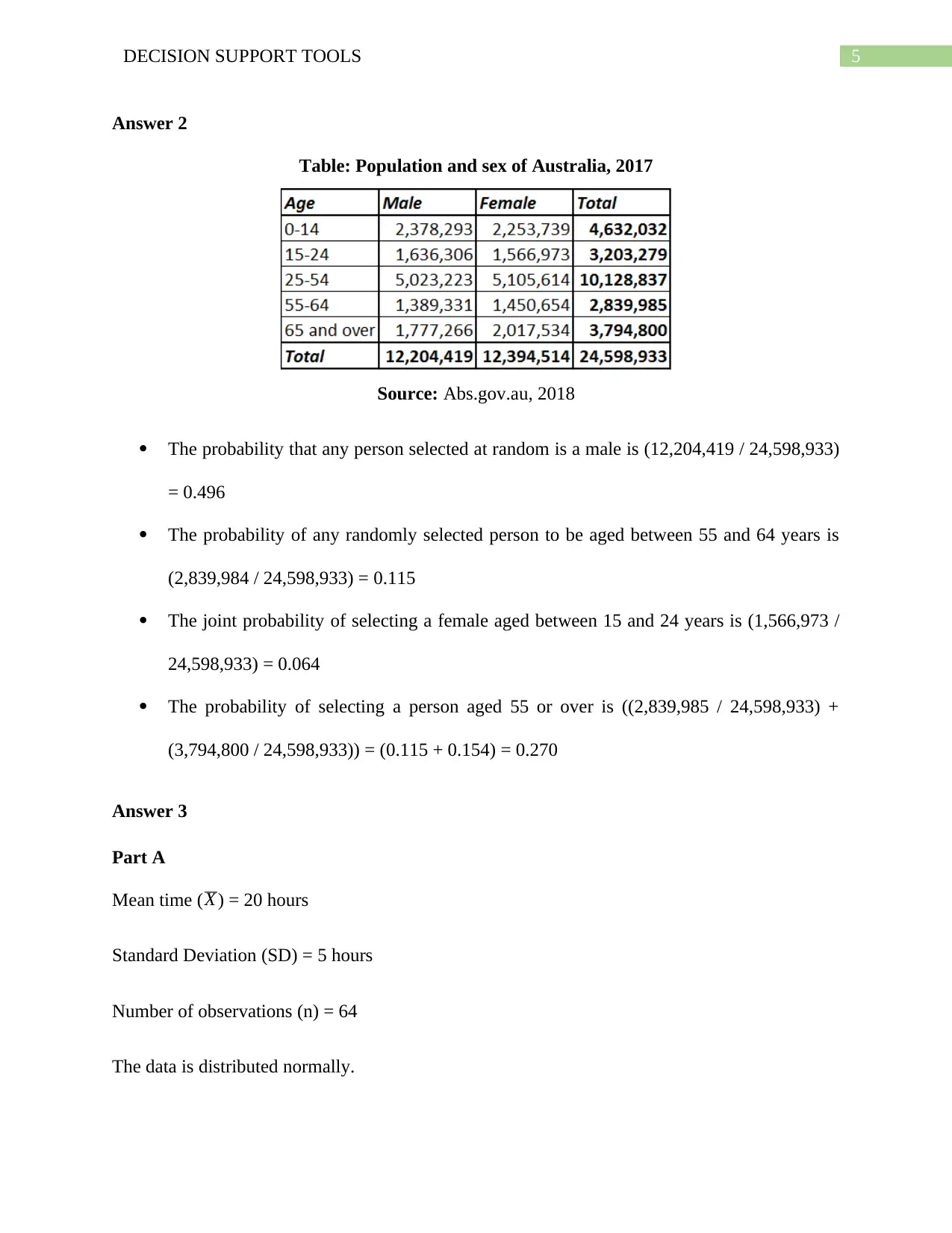
Table: Population and sex of Australia, 2017
Source: Abs.gov.au, 2018
 The probability that any person selected at random is a male is (12,204,419 / 24,598,933)
= 0.496
 The probability of any randomly selected person to be aged between 55 and 64 years is
(2,839,984 / 24,598,933) = 0.115
 The joint probability of selecting a female aged between 15 and 24 years is (1,566,973 /
24,598,933) = 0.064
 The probability of selecting a person aged 55 or over is ((2,839,985 / 24,598,933) +
(3,794,800 / 24,598,933)) = (0.115 + 0.154) = 0.270
Answer 3
Part A
Mean time (X ) = 20 hours
Standard Deviation (SD) = 5 hours
Number of observations (n) = 64
The data is distributed normally.

6DECISION SUPPORT TOOLS
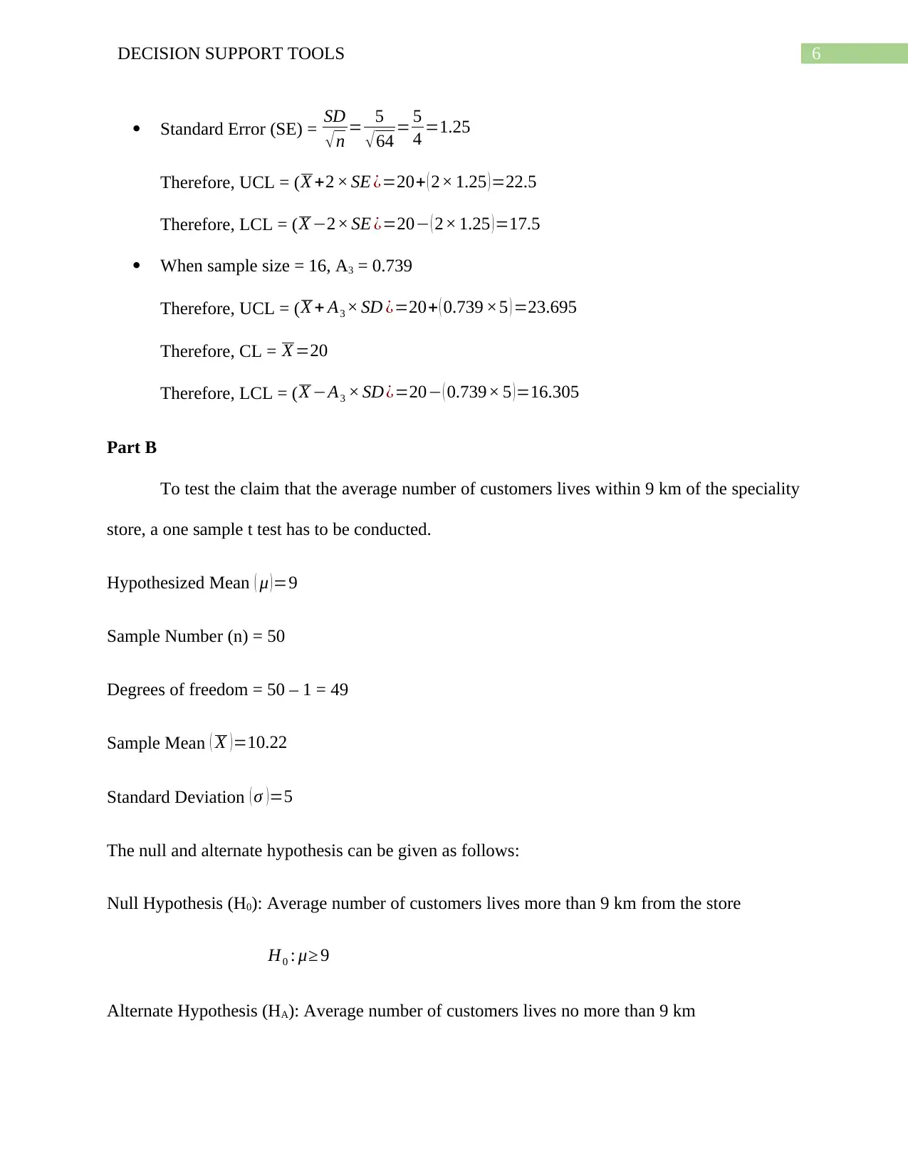
 Standard Error (SE) = SD
√ n = 5
√ 64 = 5
4 =1.25
Therefore, UCL = (X +2 × SE ¿=20+ ( 2× 1.25 )=22.5
Therefore, LCL = (X −2× SE ¿=20− ( 2× 1.25 )=17.5
 When sample size = 16, A3 = 0.739
Therefore, UCL = ( X + A3 × SD ¿=20+ ( 0.739 ×5 ) =23.695
Therefore, CL = X =20
Therefore, LCL = ( X −A3 × SD ¿=20− ( 0.739× 5 ) =16.305
Part B
To test the claim that the average number of customers lives within 9 km of the speciality
store, a one sample t test has to be conducted.
Hypothesized Mean ( μ ) =9
Sample Number (n) = 50
Degrees of freedom = 50 – 1 = 49
Sample Mean ( X )=10.22
Standard Deviation ( σ )=5
The null and alternate hypothesis can be given as follows:
Null Hypothesis (H0): Average number of customers lives more than 9 km from the store
H0 : μ≥ 9
Alternate Hypothesis (HA): Average number of customers lives no more than 9 km

7DECISION SUPPORT TOOLS
H A : μ<9
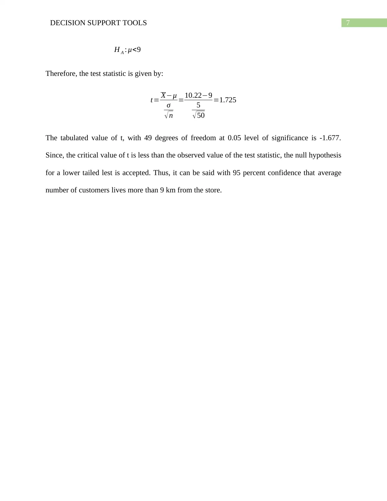
Therefore, the test statistic is given by:
t= X−μ
σ
√n
=10.22−9
5
√50
=1.725
The tabulated value of t, with 49 degrees of freedom at 0.05 level of significance is -1.677.
Since, the critical value of t is less than the observed value of the test statistic, the null hypothesis
for a lower tailed lest is accepted. Thus, it can be said with 95 percent confidence that average
number of customers lives more than 9 km from the store.

8DECISION SUPPORT TOOLS
References
3101.0 - Australian Demographic Statistics, Jun 2017. (2018). Abs.gov.au. Retrieved 12 March
2018, from http://www.abs.gov.au/AUSSTATS/abs@.nsf/DetailsPage/3101.0Jun
%202017?OpenDocument
Rohatgi, V. K., & Saleh, A. M. E. (2015). An introduction to probability and statistics. John
Wiley & Sons.