Desklib Online Library for Study Material with Solved Assignments

This article covers topics related to applied quantitative methods, measures of variability and association, linear regression, and probability. It includes solved assignments and questions related to these topics. The article also mentions Desklib, an online library for study material with solved assignments, essays, dissertations, etc.

HA1011 – Applied Quantitative Methods
Group Assignment
Attempt all the questions (8x2.5 = 20 Marks)
Question 1 of 8
HINT: We cover this in Lecture 1(Summary Statistics and Graphs)
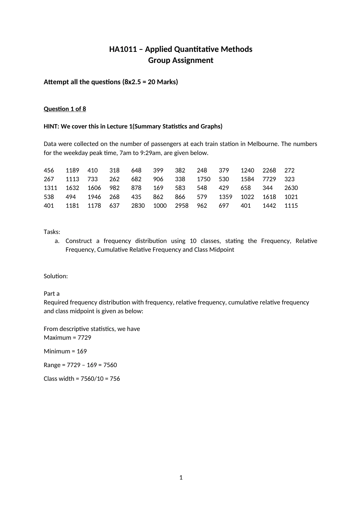
Data were collected on the number of passengers at each train station in Melbourne. The numbers
for the weekday peak time, 7am to 9:29am, are given below.
456 1189 410 318 648 399 382 248 379 1240 2268 272
267 1113 733 262 682 906 338 1750 530 1584 7729 323
1311 1632 1606 982 878 169 583 548 429 658 344 2630
538 494 1946 268 435 862 866 579 1359 1022 1618 1021
401 1181 1178 637 2830 1000 2958 962 697 401 1442 1115
Tasks:
a. Construct a frequency distribution using 10 classes, stating the Frequency, Relative
Frequency, Cumulative Relative Frequency and Class Midpoint
Solution:
Part a
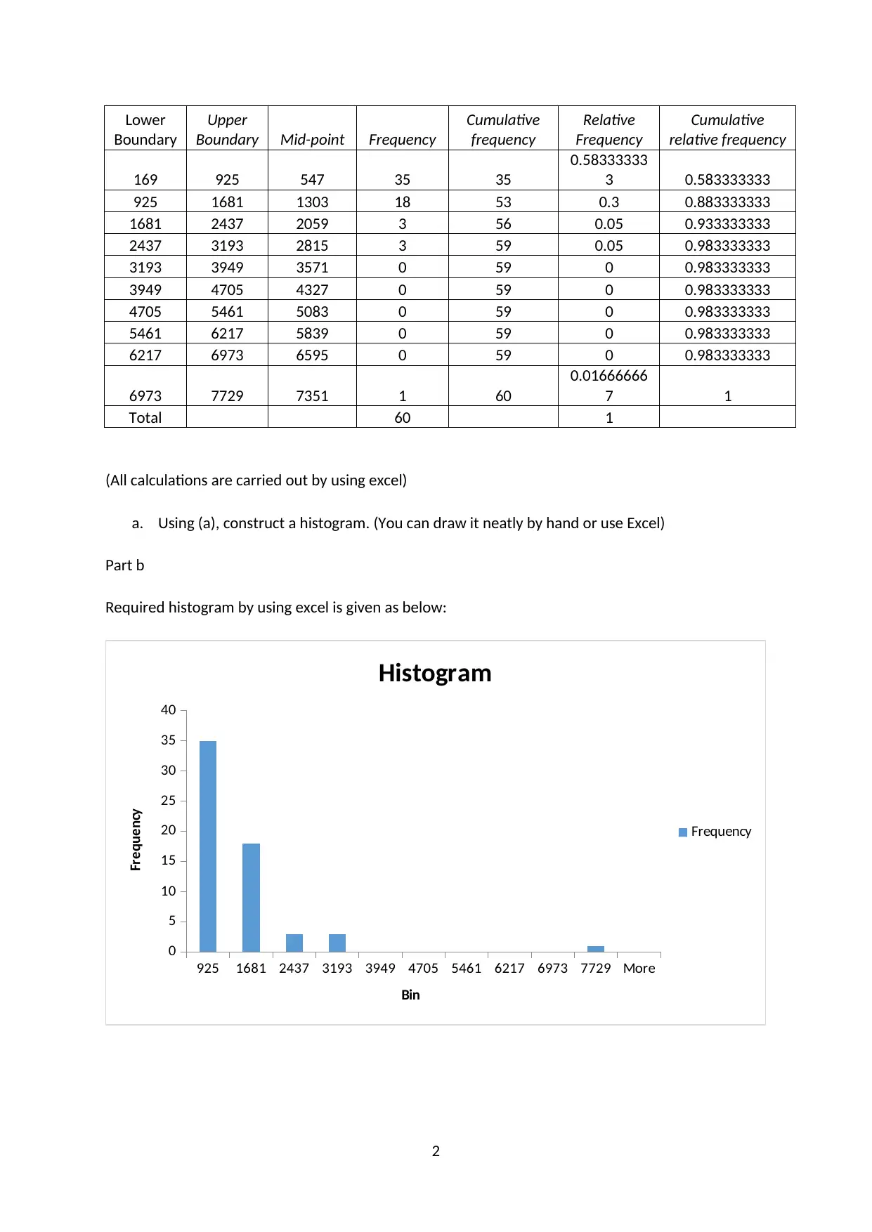
Required frequency distribution with frequency, relative frequency, cumulative relative frequency
and class midpoint is given as below:
From descriptive statistics, we have
Maximum = 7729
Minimum = 169
Range = 7729 – 169 = 7560
Class width = 7560/10 = 756
1

Lower
Boundary
Upper
Boundary Mid-point Frequency
Cumulative
frequency
Relative
Frequency
Cumulative
relative frequency
169 925 547 35 35
0.58333333
3 0.583333333
925 1681 1303 18 53 0.3 0.883333333
1681 2437 2059 3 56 0.05 0.933333333
2437 3193 2815 3 59 0.05 0.983333333
3193 3949 3571 0 59 0 0.983333333
3949 4705 4327 0 59 0 0.983333333
4705 5461 5083 0 59 0 0.983333333
5461 6217 5839 0 59 0 0.983333333
6217 6973 6595 0 59 0 0.983333333
6973 7729 7351 1 60
0.01666666
7 1
Total 60 1
(All calculations are carried out by using excel)
a. Using (a), construct a histogram. (You can draw it neatly by hand or use Excel)
Part b
Required histogram by using excel is given as below:
925 1681 2437 3193 3949 4705 5461 6217 6973 7729 More
0
5
10
15
20
25
30
35
40
Histogram
Frequency
Bin
Frequency
2

a. Based upon the raw data (NOT the Frequency Distribution), what is the mean, median and
mode? (Hint – first sort your data. This is usually much easier using Excel.)
Part c
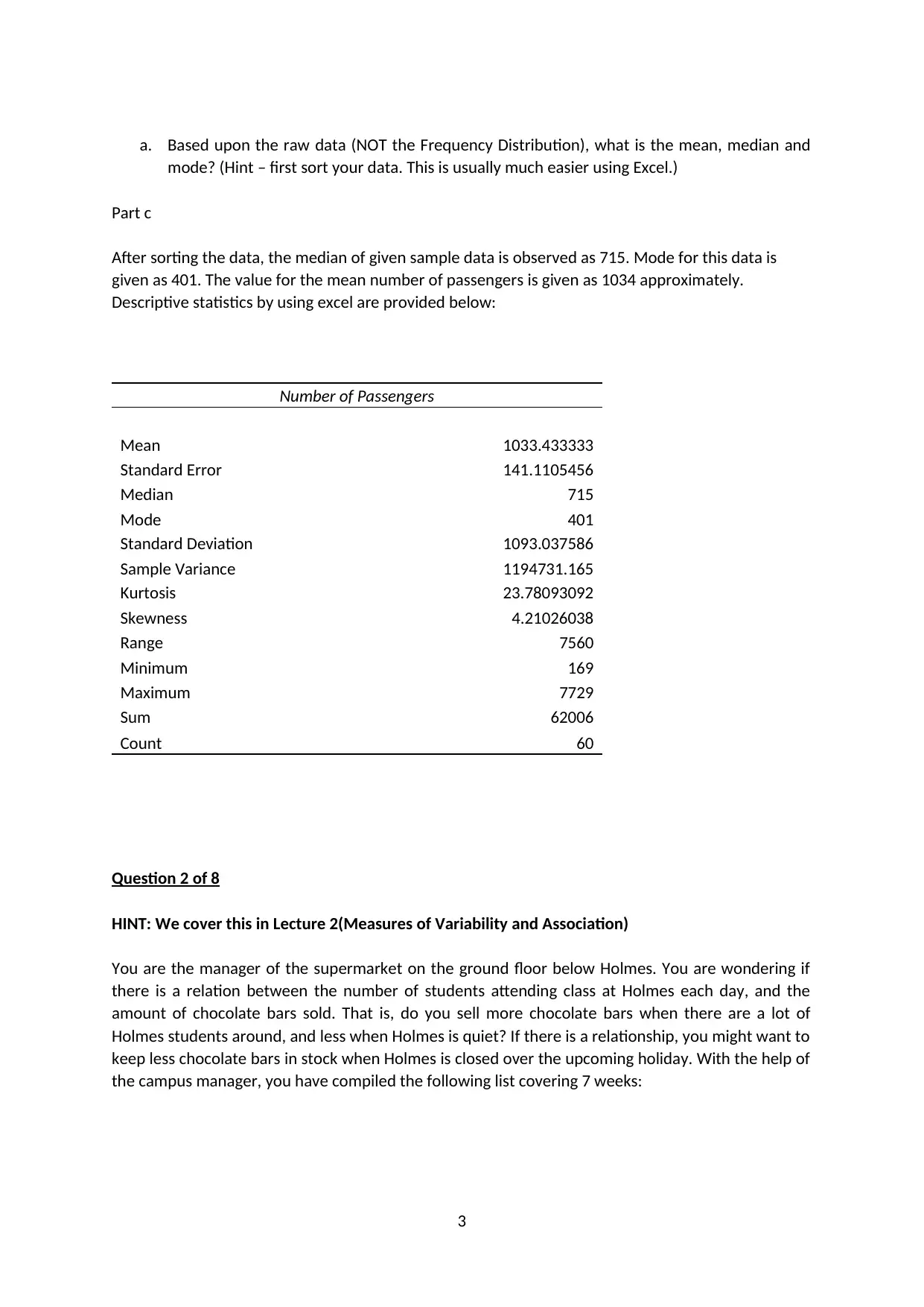
After sorting the data, the median of given sample data is observed as 715. Mode for this data is
given as 401. The value for the mean number of passengers is given as 1034 approximately.
Descriptive statistics by using excel are provided below:
Number of Passengers
Mean 1033.433333
Standard Error 141.1105456
Median 715
Mode 401
Standard Deviation 1093.037586
Sample Variance 1194731.165
Kurtosis 23.78093092
Skewness 4.21026038
Range 7560
Minimum 169
Maximum 7729
Sum 62006
Count 60
Question 2 of 8
HINT: We cover this in Lecture 2(Measures of Variability and Association)
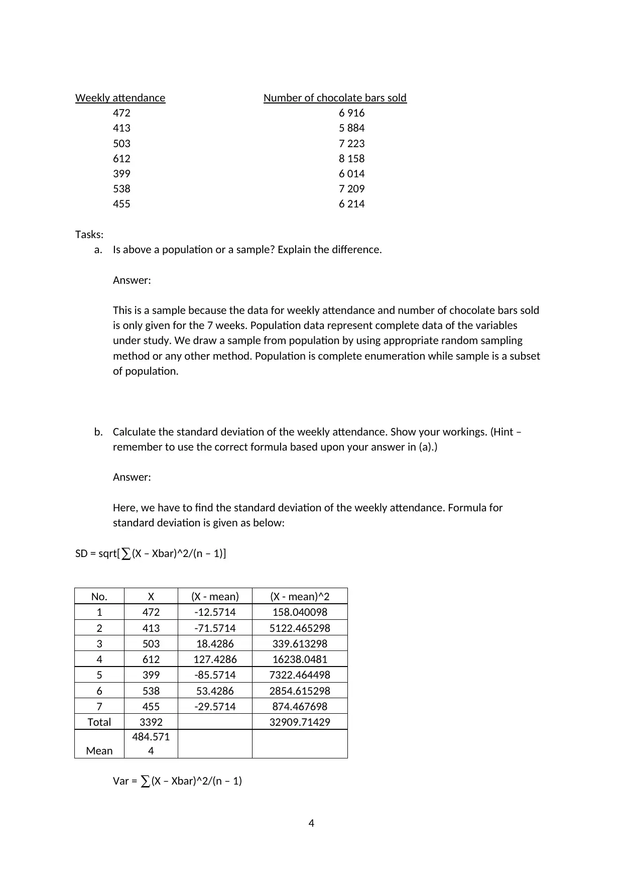
You are the manager of the supermarket on the ground floor below Holmes. You are wondering if
there is a relation between the number of students attending class at Holmes each day, and the
amount of chocolate bars sold. That is, do you sell more chocolate bars when there are a lot of
Holmes students around, and less when Holmes is quiet? If there is a relationship, you might want to
keep less chocolate bars in stock when Holmes is closed over the upcoming holiday. With the help of
the campus manager, you have compiled the following list covering 7 weeks:
3

Weekly attendance Number of chocolate bars sold
472 6 916
413 5 884
503 7 223
612 8 158
399 6 014
538 7 209
455 6 214
Tasks:
a. Is above a population or a sample? Explain the difference.
Answer:
This is a sample because the data for weekly attendance and number of chocolate bars sold
is only given for the 7 weeks. Population data represent complete data of the variables
under study. We draw a sample from population by using appropriate random sampling
method or any other method. Population is complete enumeration while sample is a subset
of population.
b. Calculate the standard deviation of the weekly attendance. Show your workings. (Hint –
remember to use the correct formula based upon your answer in (a).)
Answer:
Here, we have to find the standard deviation of the weekly attendance. Formula for
standard deviation is given as below:
SD = sqrt[∑(X – Xbar)^2/(n – 1)]
No. X (X - mean) (X - mean)^2
1 472 -12.5714 158.040098
2 413 -71.5714 5122.465298
3 503 18.4286 339.613298
4 612 127.4286 16238.0481
5 399 -85.5714 7322.464498
6 538 53.4286 2854.615298
7 455 -29.5714 874.467698
Total 3392 32909.71429
Mean
484.571
4
Var = ∑(X – Xbar)^2/(n – 1)
4

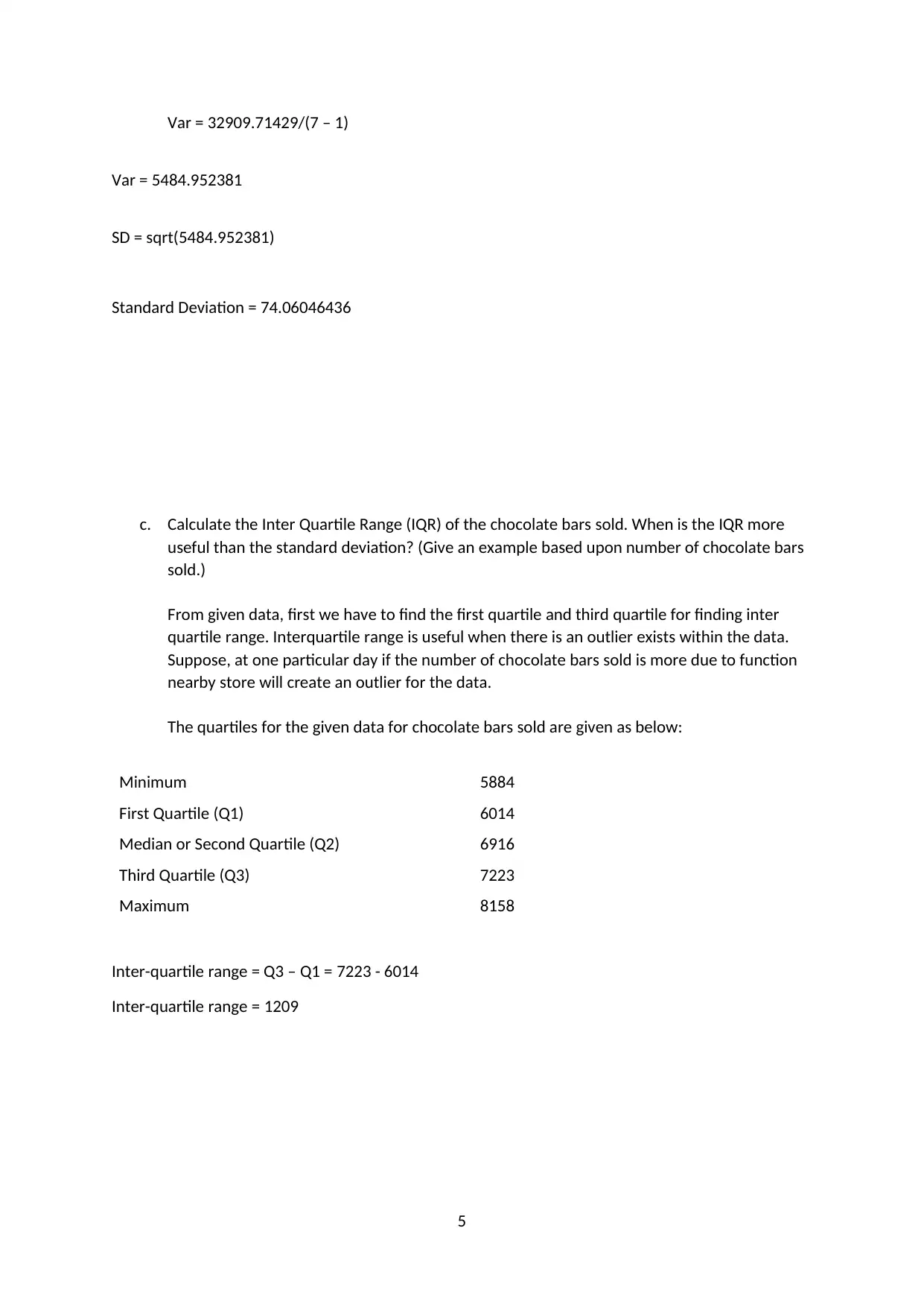
Var = 32909.71429/(7 – 1)
Var = 5484.952381
SD = sqrt(5484.952381)
Standard Deviation = 74.06046436
c. Calculate the Inter Quartile Range (IQR) of the chocolate bars sold. When is the IQR more
useful than the standard deviation? (Give an example based upon number of chocolate bars
sold.)
From given data, first we have to find the first quartile and third quartile for finding inter
quartile range. Interquartile range is useful when there is an outlier exists within the data.
Suppose, at one particular day if the number of chocolate bars sold is more due to function
nearby store will create an outlier for the data.
The quartiles for the given data for chocolate bars sold are given as below:
Minimum 5884
First Quartile (Q1) 6014
Median or Second Quartile (Q2) 6916
Third Quartile (Q3) 7223
Maximum 8158
Inter-quartile range = Q3 – Q1 = 7223 - 6014
Inter-quartile range = 1209
5

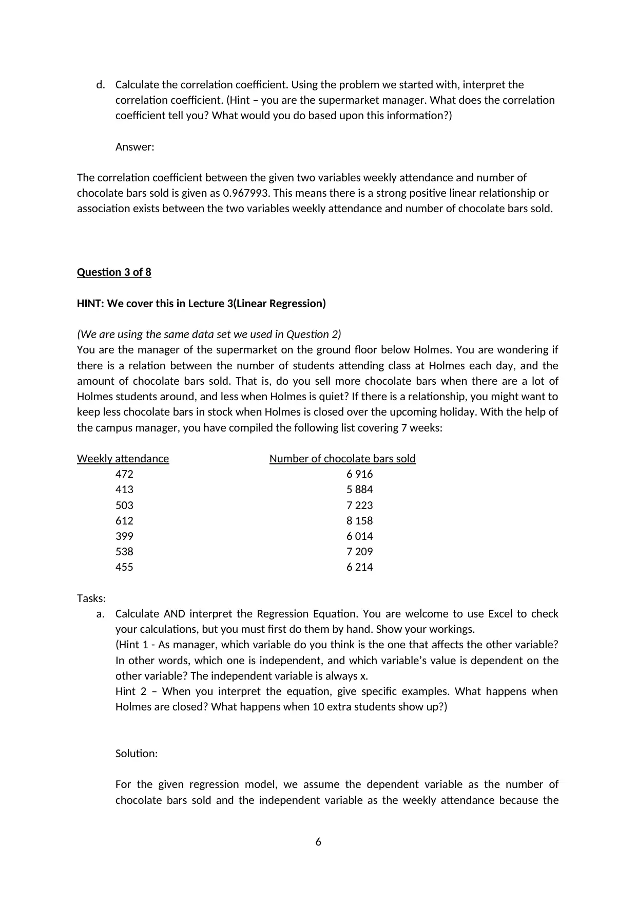
d. Calculate the correlation coefficient. Using the problem we started with, interpret the
correlation coefficient. (Hint – you are the supermarket manager. What does the correlation
coefficient tell you? What would you do based upon this information?)
Answer:
The correlation coefficient between the given two variables weekly attendance and number of
chocolate bars sold is given as 0.967993. This means there is a strong positive linear relationship or
association exists between the two variables weekly attendance and number of chocolate bars sold.
Question 3 of 8
HINT: We cover this in Lecture 3(Linear Regression)
(We are using the same data set we used in Question 2)
You are the manager of the supermarket on the ground floor below Holmes. You are wondering if
there is a relation between the number of students attending class at Holmes each day, and the
amount of chocolate bars sold. That is, do you sell more chocolate bars when there are a lot of
Holmes students around, and less when Holmes is quiet? If there is a relationship, you might want to
keep less chocolate bars in stock when Holmes is closed over the upcoming holiday. With the help of
the campus manager, you have compiled the following list covering 7 weeks:
Weekly attendance Number of chocolate bars sold
472 6 916
413 5 884
503 7 223
612 8 158
399 6 014
538 7 209
455 6 214
Tasks:
a. Calculate AND interpret the Regression Equation. You are welcome to use Excel to check
your calculations, but you must first do them by hand. Show your workings.
(Hint 1 - As manager, which variable do you think is the one that affects the other variable?
In other words, which one is independent, and which variable’s value is dependent on the
other variable? The independent variable is always x.
Hint 2 – When you interpret the equation, give specific examples. What happens when
Holmes are closed? What happens when 10 extra students show up?)
Solution:
For the given regression model, we assume the dependent variable as the number of
chocolate bars sold and the independent variable as the weekly attendance because the
6

number of chocolate bars sold are depends upon the weekly attendance of the students at
Holmes.
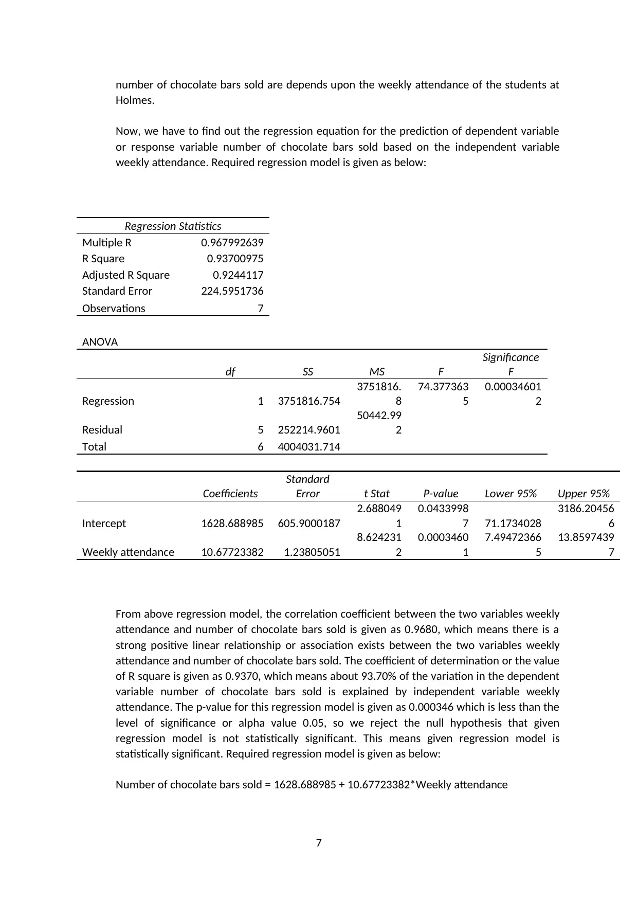
Now, we have to find out the regression equation for the prediction of dependent variable
or response variable number of chocolate bars sold based on the independent variable
weekly attendance. Required regression model is given as below:
Regression Statistics
Multiple R 0.967992639
R Square 0.93700975
Adjusted R Square 0.9244117
Standard Error 224.5951736
Observations 7
ANOVA
df SS MS F
Significance
F
Regression 1 3751816.754
3751816.
8
74.377363
5
0.00034601
2
Residual 5 252214.9601
50442.99
2
Total 6 4004031.714
Coefficients
Standard
Error t Stat P-value Lower 95% Upper 95%
Intercept 1628.688985 605.9000187
2.688049
1
0.0433998
7 71.1734028
3186.20456
6
Weekly attendance 10.67723382 1.23805051
8.624231
2
0.0003460
1
7.49472366
5
13.8597439
7
From above regression model, the correlation coefficient between the two variables weekly
attendance and number of chocolate bars sold is given as 0.9680, which means there is a
strong positive linear relationship or association exists between the two variables weekly
attendance and number of chocolate bars sold. The coefficient of determination or the value
of R square is given as 0.9370, which means about 93.70% of the variation in the dependent
variable number of chocolate bars sold is explained by independent variable weekly
attendance. The p-value for this regression model is given as 0.000346 which is less than the
level of significance or alpha value 0.05, so we reject the null hypothesis that given
regression model is not statistically significant. This means given regression model is
statistically significant. Required regression model is given as below:
Number of chocolate bars sold = 1628.688985 + 10.67723382*Weekly attendance
7

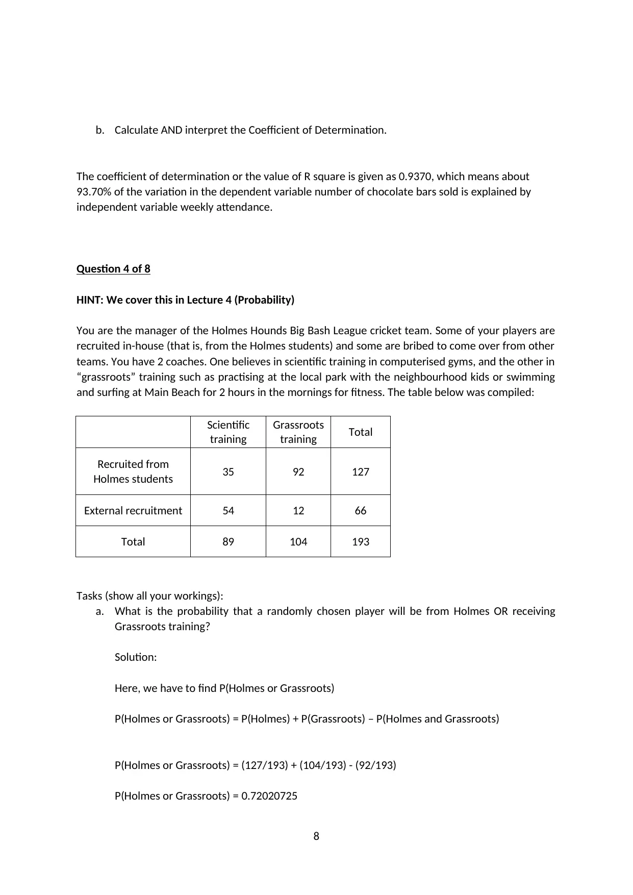
b. Calculate AND interpret the Coefficient of Determination.
The coefficient of determination or the value of R square is given as 0.9370, which means about
93.70% of the variation in the dependent variable number of chocolate bars sold is explained by
independent variable weekly attendance.
Question 4 of 8
HINT: We cover this in Lecture 4 (Probability)
You are the manager of the Holmes Hounds Big Bash League cricket team. Some of your players are
recruited in-house (that is, from the Holmes students) and some are bribed to come over from other
teams. You have 2 coaches. One believes in scientific training in computerised gyms, and the other in
“grassroots” training such as practising at the local park with the neighbourhood kids or swimming
and surfing at Main Beach for 2 hours in the mornings for fitness. The table below was compiled:
Scientific
training
Grassroots
training Total
Recruited from
Holmes students 35 92 127
External recruitment 54 12 66
Total 89 104 193
Tasks (show all your workings):
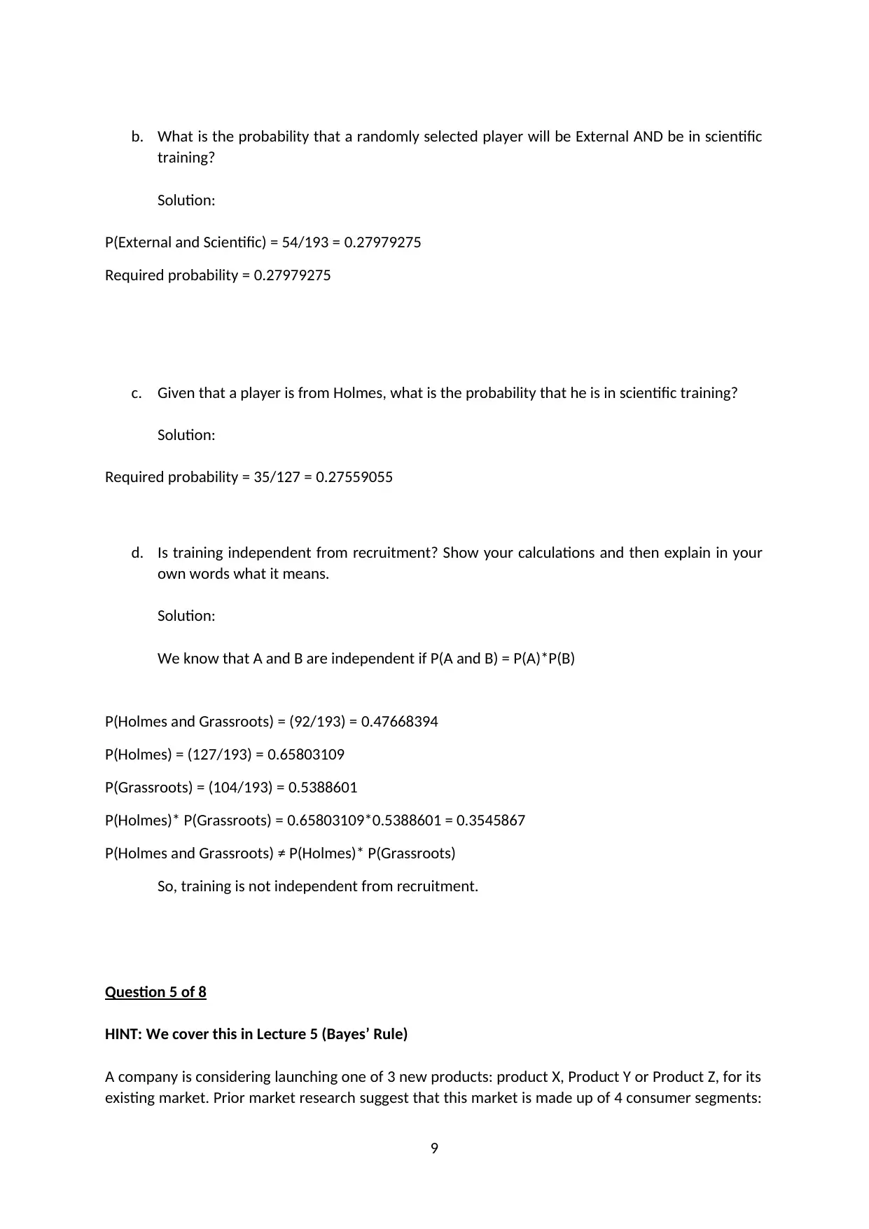
a. What is the probability that a randomly chosen player will be from Holmes OR receiving
Grassroots training?
Solution:
Here, we have to find P(Holmes or Grassroots)
P(Holmes or Grassroots) = P(Holmes) + P(Grassroots) – P(Holmes and Grassroots)
P(Holmes or Grassroots) = (127/193) + (104/193) - (92/193)
P(Holmes or Grassroots) = 0.72020725
8

b. What is the probability that a randomly selected player will be External AND be in scientific
training?
Solution:
P(External and Scientific) = 54/193 = 0.27979275
Required probability = 0.27979275
c. Given that a player is from Holmes, what is the probability that he is in scientific training?
Solution:
Required probability = 35/127 = 0.27559055
d. Is training independent from recruitment? Show your calculations and then explain in your
own words what it means.
Solution:
We know that A and B are independent if P(A and B) = P(A)*P(B)
P(Holmes and Grassroots) = (92/193) = 0.47668394
P(Holmes) = (127/193) = 0.65803109
P(Grassroots) = (104/193) = 0.5388601
P(Holmes)* P(Grassroots) = 0.65803109*0.5388601 = 0.3545867
P(Holmes and Grassroots) ≠ P(Holmes)* P(Grassroots)
So, training is not independent from recruitment.
Question 5 of 8
HINT: We cover this in Lecture 5 (Bayes’ Rule)
A company is considering launching one of 3 new products: product X, Product Y or Product Z, for its
existing market. Prior market research suggest that this market is made up of 4 consumer segments:
9

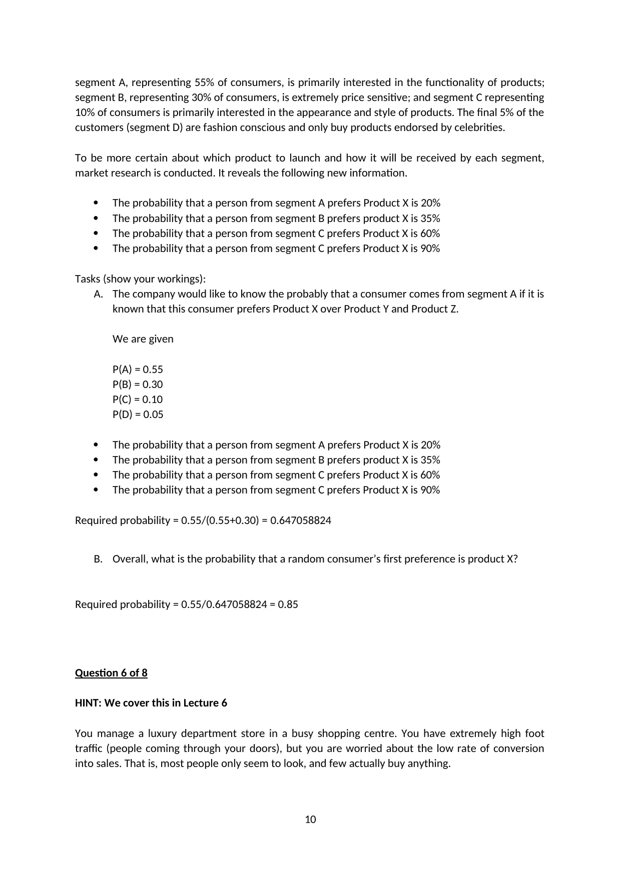
segment A, representing 55% of consumers, is primarily interested in the functionality of products;
segment B, representing 30% of consumers, is extremely price sensitive; and segment C representing
10% of consumers is primarily interested in the appearance and style of products. The final 5% of the
customers (segment D) are fashion conscious and only buy products endorsed by celebrities.
To be more certain about which product to launch and how it will be received by each segment,
market research is conducted. It reveals the following new information.
 The probability that a person from segment A prefers Product X is 20%
 The probability that a person from segment B prefers product X is 35%
 The probability that a person from segment C prefers Product X is 60%
 The probability that a person from segment C prefers Product X is 90%
Tasks (show your workings):
A. The company would like to know the probably that a consumer comes from segment A if it is
known that this consumer prefers Product X over Product Y and Product Z.
We are given
P(A) = 0.55
P(B) = 0.30
P(C) = 0.10
P(D) = 0.05
 The probability that a person from segment A prefers Product X is 20%
 The probability that a person from segment B prefers product X is 35%
 The probability that a person from segment C prefers Product X is 60%
 The probability that a person from segment C prefers Product X is 90%
Required probability = 0.55/(0.55+0.30) = 0.647058824
B. Overall, what is the probability that a random consumer’s first preference is product X?
Required probability = 0.55/0.647058824 = 0.85
Question 6 of 8
HINT: We cover this in Lecture 6
You manage a luxury department store in a busy shopping centre. You have extremely high foot
traffic (people coming through your doors), but you are worried about the low rate of conversion
into sales. That is, most people only seem to look, and few actually buy anything.
10

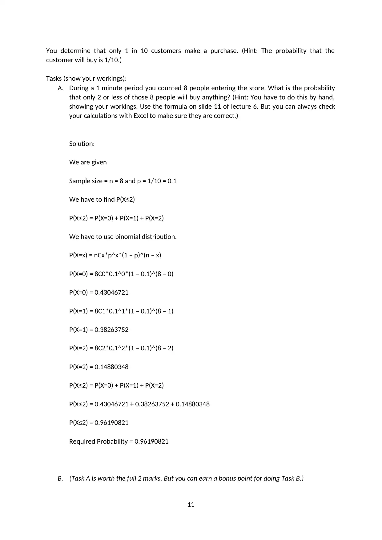
You determine that only 1 in 10 customers make a purchase. (Hint: The probability that the
customer will buy is 1/10.)
Tasks (show your workings):
A. During a 1 minute period you counted 8 people entering the store. What is the probability
that only 2 or less of those 8 people will buy anything? (Hint: You have to do this by hand,
showing your workings. Use the formula on slide 11 of lecture 6. But you can always check
your calculations with Excel to make sure they are correct.)
Solution:
We are given
Sample size = n = 8 and p = 1/10 = 0.1
We have to find P(X≤2)
P(X≤2) = P(X=0) + P(X=1) + P(X=2)
We have to use binomial distribution.
P(X=x) = nCx*p^x*(1 – p)^(n – x)
P(X=0) = 8C0*0.1^0*(1 – 0.1)^(8 – 0)
P(X=0) = 0.43046721
P(X=1) = 8C1*0.1^1*(1 – 0.1)^(8 – 1)
P(X=1) = 0.38263752
P(X=2) = 8C2*0.1^2*(1 – 0.1)^(8 – 2)
P(X=2) = 0.14880348
P(X≤2) = P(X=0) + P(X=1) + P(X=2)
P(X≤2) = 0.43046721 + 0.38263752 + 0.14880348
P(X≤2) = 0.96190821
Required Probability = 0.96190821
B. (Task A is worth the full 2 marks. But you can earn a bonus point for doing Task B.)
11

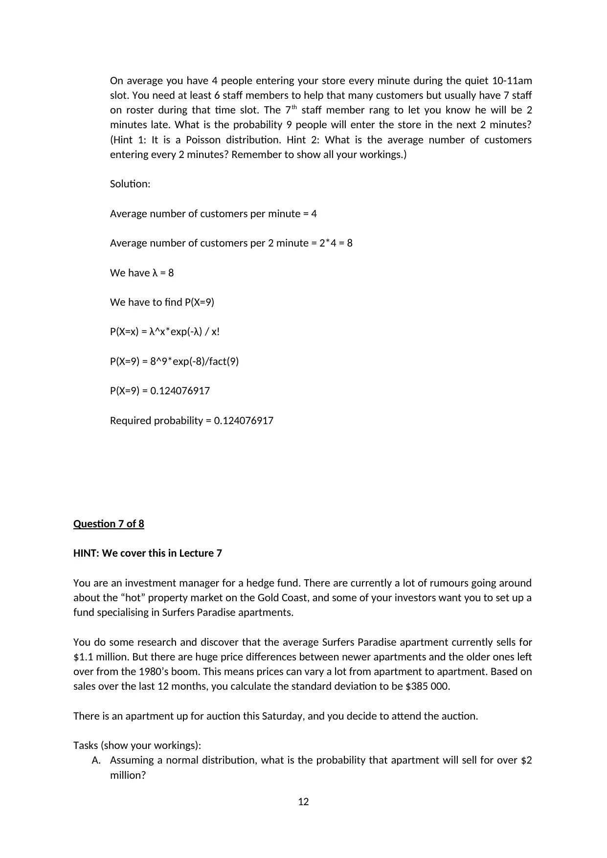
On average you have 4 people entering your store every minute during the quiet 10-11am
slot. You need at least 6 staff members to help that many customers but usually have 7 staff
on roster during that time slot. The 7th staff member rang to let you know he will be 2
minutes late. What is the probability 9 people will enter the store in the next 2 minutes?
(Hint 1: It is a Poisson distribution. Hint 2: What is the average number of customers
entering every 2 minutes? Remember to show all your workings.)
Solution:
Average number of customers per minute = 4
Average number of customers per 2 minute = 2*4 = 8
We have λ = 8
We have to find P(X=9)
P(X=x) = λ^x*exp(-λ) / x!
P(X=9) = 8^9*exp(-8)/fact(9)
P(X=9) = 0.124076917
Required probability = 0.124076917
Question 7 of 8
HINT: We cover this in Lecture 7
You are an investment manager for a hedge fund. There are currently a lot of rumours going around
about the “hot” property market on the Gold Coast, and some of your investors want you to set up a
fund specialising in Surfers Paradise apartments.
You do some research and discover that the average Surfers Paradise apartment currently sells for
$1.1 million. But there are huge price differences between newer apartments and the older ones left
over from the 1980’s boom. This means prices can vary a lot from apartment to apartment. Based on
sales over the last 12 months, you calculate the standard deviation to be $385 000.
There is an apartment up for auction this Saturday, and you decide to attend the auction.
Tasks (show your workings):
A. Assuming a normal distribution, what is the probability that apartment will sell for over $2
million?
12

We are given
Mean = 1.1 million
SD = 385000 = 0.385 million
We have to find P(X>2)
P(X>2) = 1 – P(X<2)
Z = (X – mean) / SD
Z = (2 – 1.1) / 0.385
Z = 2.337662338
P(Z<2.337662338) = 0.990297614
P(X<2) = 0.990297614
P(X>2) = 1 – P(X<2)
P(X>2) = 1 – 0.990297614
P(X>2) = 0.009702386
Required probability = 0.009702386
B. What is the probability that the apartment will sell for over $1 million but less than $1.1
million?
Solution:
Here, we have to find P(1<X<1.1)
P(1<X<1.1) = P(X<1.1) – P(X<1)
We are given
Mean = 1.1 million
SD = 385000 = 0.385 million
First we have to find P(X<1.1)
13

Z = (1.1 – 1.1) / 0.385
Z = 0
P(Z<0) = 0.50
P(X<1.1) = 0.50
Now, we have to find P(X<1)
Z = (1 – 1.1) / 0.385
Z = -0.25974026
P(Z< -0.25974026) = 0.397532068
P(X<1) = 0.397532068
P(1<X<1.1) = P(X<1.1) – P(X<1)
P(1<X<1.1) = 0.50 - 0.397532068
P(1<X<1.1) = 0.102467932
Required probability = 0.102467932
Question 8 of 8
HINT: We cover this in Lecture 8
You are an investment manager for a hedge fund. There are currently a lot of rumours going around
about the “hot” property market on the Gold Coast, and some of your investors want you to set up a
fund specialising in Surfers Paradise apartments.
Last Saturday you attended an auction to get “a feel” for the local real estate market. You decide it
might be worth further investigating. You ask one of your interns to take a quick sample of 50
properties that have been sold during the last few months. Your previous research indicated an
average price of $1.1 million but the average price of your assistant’s sample was only $950 000.
However, the standard deviation for her research was the same as yours at $385 000.
Tasks (show your workings):
A. Since the apartments on Surfers Paradise are a mix of cheap older and more expensive new
apartments, you know the distribution is NOT normal. Can you still use a Z-distribution to
test your assistant’s research findings against yours? Why, or why not?
Answer:
14

Yes, still we can use a Z-distribution to test assistant’s research findings against previous
findings, because a sample size selected by assistant is 50 and this sample size is adequate
for using normal distribution (n>30) and also we know that the sampling distribution of any
sample statistic follows an approximately normal distribution although given sample follows
or not follows a normal distribution.
B. You have over 2 000 investors in your fund. You and your assistant phone 45 of them to ask
if they are willing to invest more than $1 million (each) to the proposed new fund. Only 11
say that they would, but you need at least 30% of your investors to participate to make the
fund profitable. Based on your sample of 45 investors, what is the probability that 30% of
the investors would be willing to commit $1 million or more to the fund?
Solution:
We are given
Sample size = N = 45
Number of successes = X = 11
Estimate for proportion = p = X/N = 11/45 = 0.244444444
Total number of investors = n = 2000
30% of 2000 investors = 600 investors
Here, we have to use normal approximation to binomial distribution.
We have to find P(X>600)
Mean = n*p = 2000*0.244444444 = 488.888888
q = 1 – p = 1 - 0.244444444 = 0.755555556
SD = sqrt(n*p*q) = sqrt(2000*0.244444444*0.755555556)
SD = 19.21933182
P(X>600) = 1 – P(X<600)
Z = (X – mean) / SD
Z = (600 - 488.888888) / 19.21933182
Z = 5.781216175
P(Z<5.781216175) = 0.999999996
P(X<600) = 0.999999996
P(X>600) = 1 – P(X<600)
P(X>600) = 1 – 0.999999996
15

P(X>600) = 0.000000001
Required probability = = 0.000000001
16