Analysis of Two Degree of Freedom Systems

This assignment delves into the analysis of a Two Degree of Freedom (2DOF) system utilizing MATLAB Simulink. It focuses on constructing mathematical models using Laplace transforms, deriving transfer functions to represent the system's behavior, and evaluating the suspension performance characteristics. The analysis includes a comparison with simpler One Degree of Freedom (1DOF) systems, highlighting the advantages and complexities introduced by the additional degrees of freedom.

Dynamic System Modelling and Control

Executive summary
A model is an accurate description of a system's dynamics. And it is mainly used to
explain the questions through the simulation and analysis. The Method of dynamic system
modelling and control is a research area of current technology. The development of modelling
and control of a motorbike performance is controlled by many parameters and have many basis.
And the motorbike have the advantages of security and comfortability. In dynamic system
modelling process the motorbike is implemented by using matlab.The method of dynamic
system is controlled by analyzing the performance of two degree of freedom, suspension
performance, and magnification factor and variation response techniques.
1. Introduction
The method of motorbike model controlling process have many criteria. This project
explains the performance of dynamic system modelling and control of the motorbike. In any kind
of automobile system the suspension performance is widely used. Because the suspension is
mainly used to maintain the grip on the road.
The main goal of this projects to implement the techniques of two degree of freedom and to
construct the three degree of freedom system. This process will be analyzed by using mat lab
Simulink. The Laplace transform modelling equations and transfer functions will be determined
in two degree of freedom (Homer, 2014).The transmissibility factor and magnification factor will
be calculated for two degree of freedom in Simulink. The simulation process of multiple degree
of freedom will be analyzed.
1

2. Mathematical model of dynamic system
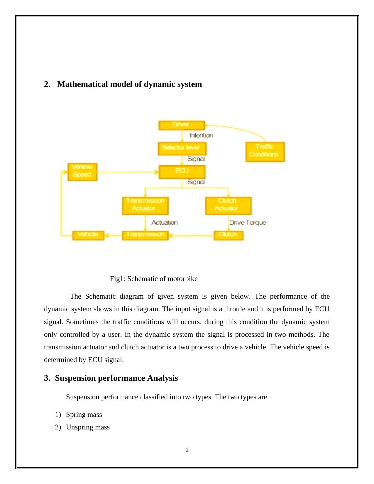
Fig1: Schematic of motorbike
The Schematic diagram of given system is given below. The performance of the
dynamic system shows in this diagram. The input signal is a throttle and it is performed by ECU
signal. Sometimes the traffic conditions will occurs, during this condition the dynamic system
only controlled by a user. In the dynamic system the signal is processed in two methods. The
transmission actuator and clutch actuator is a two process to drive a vehicle. The vehicle speed is
determined by ECU signal.
3. Suspension performance Analysis
Suspension performance classified into two types. The two types are
1) Spring mass
2) Unspring mass
2

A spring mass is main condition to support the suspension system. It is one of the part of the
vehicle (Hopkins, J. and Culpepper, 2010). The wheel bear, axles and wheel hub is directly
connected to the unspring mass. The imperfections of road is obtained by the unnecessary and
uneven force on the unspring mass. Dynamic system is divided into three types. These are Active
Suspension system, Passive Suspension system and semi active suspension system.
Active suspension system
It is important system in the suspension system. The rate of the suspension of spring can
be varied in the active suspension system. These variations make good ability to the system. It is
also known as modern suspension system.
Passive suspension system
Passive suspension is extensively used system and it is very important. The passive
suspension system also called as conventional suspension system. Compared to other suspension
system it is very popular system and low cost.
Semi-active suspension system
The semi-active suspension system is otherwise called as adaptive control system. Usage
of this system is less and this system have less power. The system provide good handling when
the motorbike running in the normal surface.
4. Two degree of freedom model
The motion of 2 DOF dynamic system will be expressed with the help of two different
co-ordinates and more than one masses are required to model this system. In other hand 1 DOF
system one mass is used to develop the model. One equation is enough to describe about 1 DOF
dynamic system. In case of 2 DOF, two equations are need to develop the dynamic system
model. To represent the motion of the system two independent co-ordinates are used. The
required equations are created with the help of mass and stiffness matrices (Berbyuk, 2007).
3

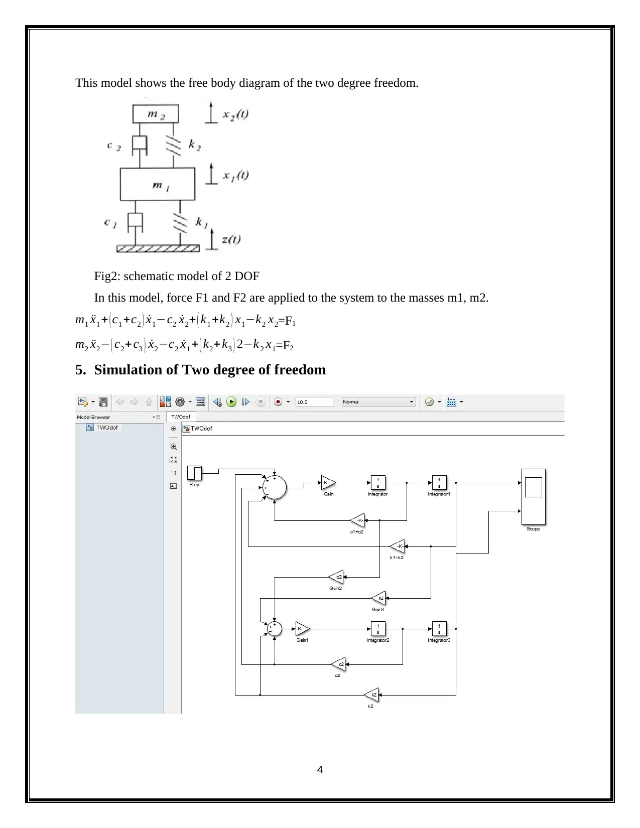
This model shows the free body diagram of the two degree freedom.
Fig2: schematic model of 2 DOF
In this model, force F1 and F2 are applied to the system to the masses m1, m2.
m1 ẍ1 + ( c1 +c2 ) ẋ1−c2 ẋ2+ ( k1 +k2 ) x1−k2 x2=F1
m2 ẍ2− ( c2+c3 ) ẋ2−c2 ẋ1 + ( k2+ k3 ) 2−k 2 x1=F2
5. Simulation of Two degree of freedom
4

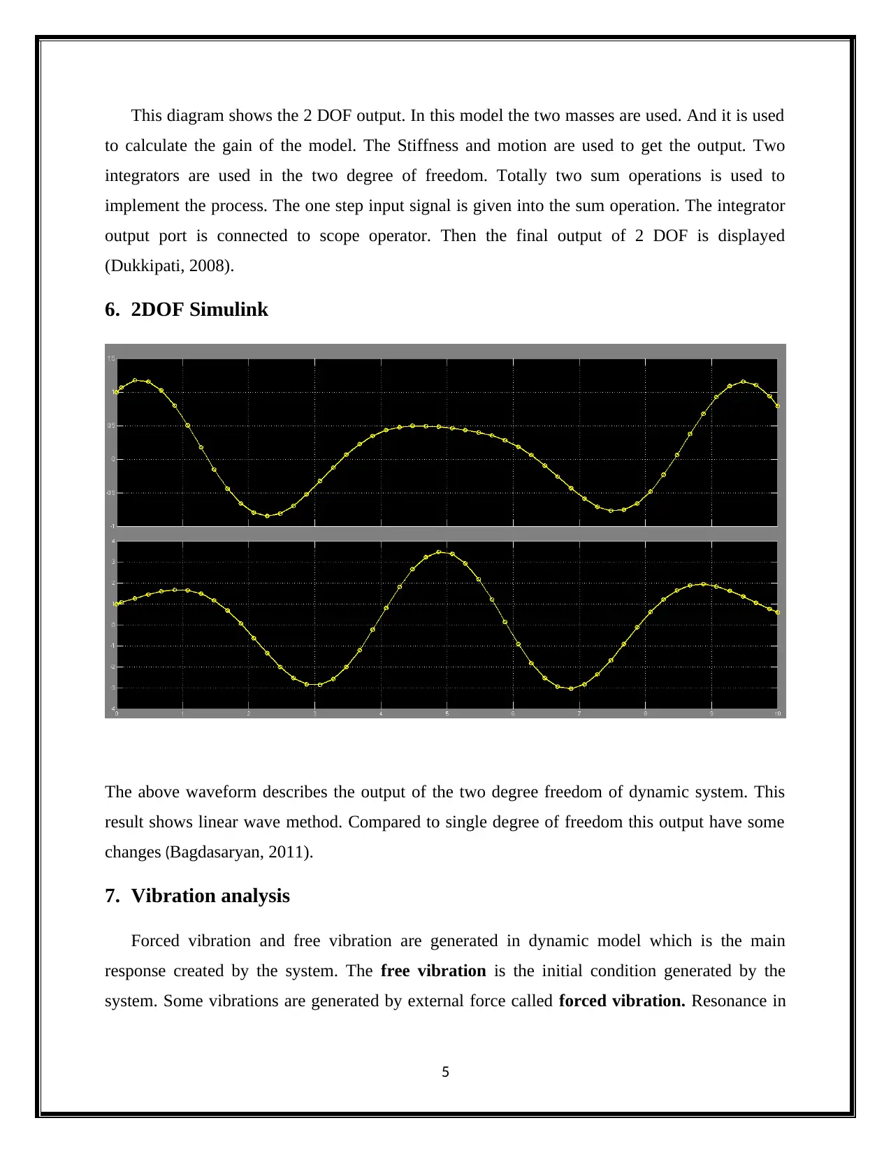
This diagram shows the 2 DOF output. In this model the two masses are used. And it is used
to calculate the gain of the model. The Stiffness and motion are used to get the output. Two
integrators are used in the two degree of freedom. Totally two sum operations is used to
implement the process. The one step input signal is given into the sum operation. The integrator
output port is connected to scope operator. Then the final output of 2 DOF is displayed
(Dukkipati, 2008).
6. 2DOF Simulink
The above waveform describes the output of the two degree freedom of dynamic system. This
result shows linear wave method. Compared to single degree of freedom this output have some
changes (Bagdasaryan, 2011).
7. Vibration analysis
Forced vibration and free vibration are generated in dynamic model which is the main
response created by the system. The free vibration is the initial condition generated by the
system. Some vibrations are generated by external force called forced vibration. Resonance in
5

the system will be occurred by some external forces. In every model external frequency and
natural frequencies are generated naturally (Buśkiewicz, 2008).
The undammed condition the equation would be,
m1 ẍ1 ( t ) + ( k1+ k2 ) x1 ( t )−k2 x2 (t )=0
m2 ẍ2 ( t ) + ( k2+ k3 ) x2 ( t ) −k 2 x1 (t)=0
This is the equation under damped condition,
m1 ( d2 x1
dt 2 ) + ( k1 + k2 ) x1−k2 x2=F1
m2 ( d2 x2
dt 2 )+ ( k 2+ k3 ) x2−k2 x1=F2
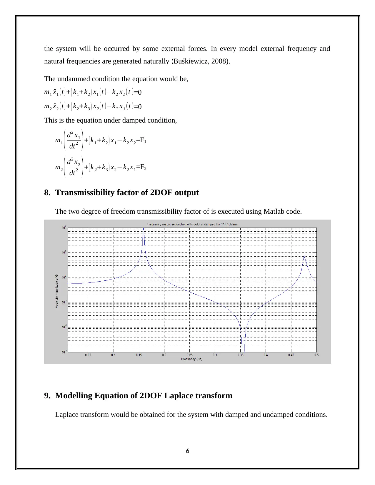
8. Transmissibility factor of 2DOF output
The two degree of freedom transmissibility factor of is executed using Matlab code.
9. Modelling Equation of 2DOF Laplace transform
Laplace transform would be obtained for the system with damped and undamped conditions.
6

For damped system the motion of the system is given by the equation which is the result of
applied force.
m1 ẍ + ( k1+ k2 ) x1−k2 x2=f 1
m1 ẍ2 + ( k 2+ k3 ) x2−k2 x2= f 2
Laplace transforms of the system when force is applied to the system.
( m1 s2+k1 +k2 ) x1−k 2 x2=F 1
( m2 s2 +k2 + K3 ) x2−k2 x1=F 2
Laplace transform for undamped condition
( m1 s2+k1 + K2 ) x1−k2 x2 =0
k 2 x1− ( m1 s2+ k1 +k2 ) x2=0
Transfer Function
The Transfer function can be obtained the using the Laplace transform of the equation. The
transfer function is defined as the ratio between Laplace transform output and the Laplace of a
system input.
x1=k2 x2 / ( m1 +k 1+ k2 )
x2=k2 x1 / ( m1 s2 +k1 + k2 )
10.Comparison between 1DOF and 2DOF
a) 2 DOF uses two different equation to develop the model but in case of 1 DOF only one
equation is enough to create the dynamic system model.
b) Compared with 2 DOF, modelling of 1 DOF system is simple.
c) Frequency response in 1DOF is ɷ=√2 s /m. In case of 2 DOF, the frequency
response of first mode is ɷ=√2 s /m. In 2 DOF second mode, the frequency response is ɷ
=√3 s /m.
Conclusion
The model of two degree of freedom has been analyzed by using Matlab Simulink. In two degree
of freedom, The Laplace transform modelling equations and transfer functions has been
7

determined the transmissibility factor was calculated for the two degree of freedom in Simulink.
The suspension performance and difference between 1 DOF and 2 DOF were discussed. The
simulation process of two degree of freedom has been done.
References
Bagdasaryan, A. (2011). Discrete dynamic simulation models and technique for complex control
systems. Simulation Modelling Practice and Theory, 19(4), pp.1061-1087.
8

Berbyuk, V. (2007). Towards dynamics of controlled multibody systems with magnetostrictive
transducers. Multibody System Dynamics, 18(2), pp.203-216.
Buśkiewicz, J. (2008). A dynamic analysis of a coupled beam/slider system. Applied
Mathematical Modelling, 32(10), pp.1941-1955.
Dukkipati, R. (2008). Control systems. Harrow, U.K.: Alpha Science International Ltd.
Homer, J. (2014). Levels of evidence in system dynamics modeling. System Dynamics Review,
30(1-2), pp.75-80.
Hopkins, J. and Culpepper, M. (2010). Synthesis of multi-degree of freedom, parallel flexure
system concepts via Freedom and Constraint Topology (FACT) – Part I: Principles. Precision
Engineering, 34(2), pp.259-270.
9

.
10