Econometrics Question and Answer 2022

Econometrics.
Econometrics.
Name
Affiliation
Date.

ECONOMETRICS.
Question 1.
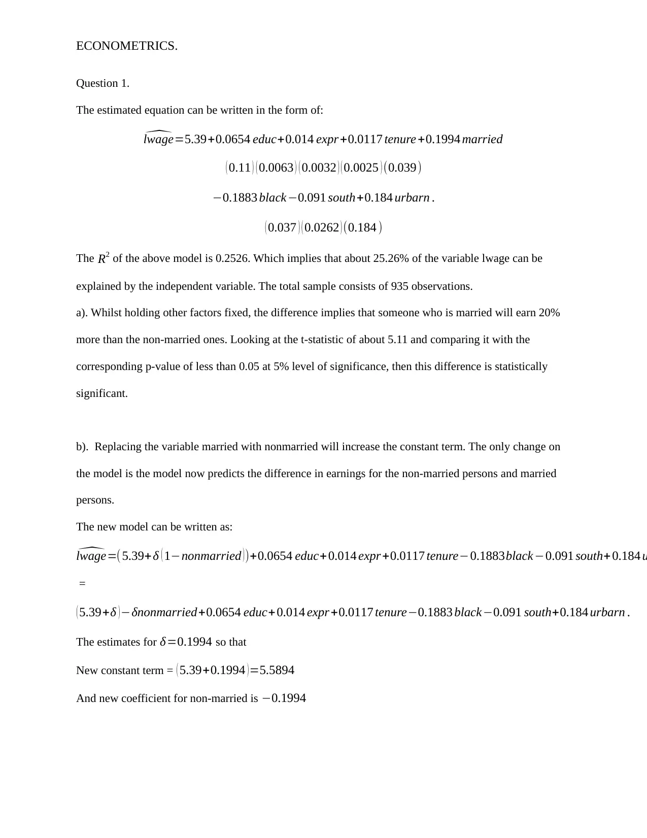
The estimated equation can be written in the form of:
^lwage=5.39+0.0654 educ+0.014 expr+0.0117 tenure +0.1994 married
( 0.11 ) ( 0.0063 ) ( 0.0032 ) ( 0.0025 ) (0.039)
−0.1883 black−0.091 south+0.184 urbarn .
( 0.037 ) ( 0.0262 ) (0.184 )
The R2 of the above model is 0.2526. Which implies that about 25.26% of the variable lwage can be
explained by the independent variable. The total sample consists of 935 observations.
a). Whilst holding other factors fixed, the difference implies that someone who is married will earn 20%
more than the non-married ones. Looking at the t-statistic of about 5.11 and comparing it with the
corresponding p-value of less than 0.05 at 5% level of significance, then this difference is statistically
significant.
b). Replacing the variable married with nonmarried will increase the constant term. The only change on
the model is the model now predicts the difference in earnings for the non-married persons and married
persons.
The new model can be written as:
^lwage=( 5.39+ δ ( 1−nonmarried ))+0.0654 educ+ 0.014 expr +0.0117 tenure−0.1883black−0.091 south+0.184 u
=
( 5.39+δ ) −δnonmarried+0.0654 educ+0.014 expr +0.0117 tenure−0.1883 black−0.091 south+0.184 urbarn .
The estimates for δ=0.1994 so that
New constant term = ( 5.39+0.1994 ) =5.5894
And new coefficient for non-married is −0.1994

ECONOMETRICS.
As a fact, the two variables married and nonmarried cannot be included both in the same model. This is
because its not possible to hold nonmarried as a constant while varying married. Inclusion of only one
variable is required, while making the other variable a reference group. This will help to avoid the dummy
variable trap1.
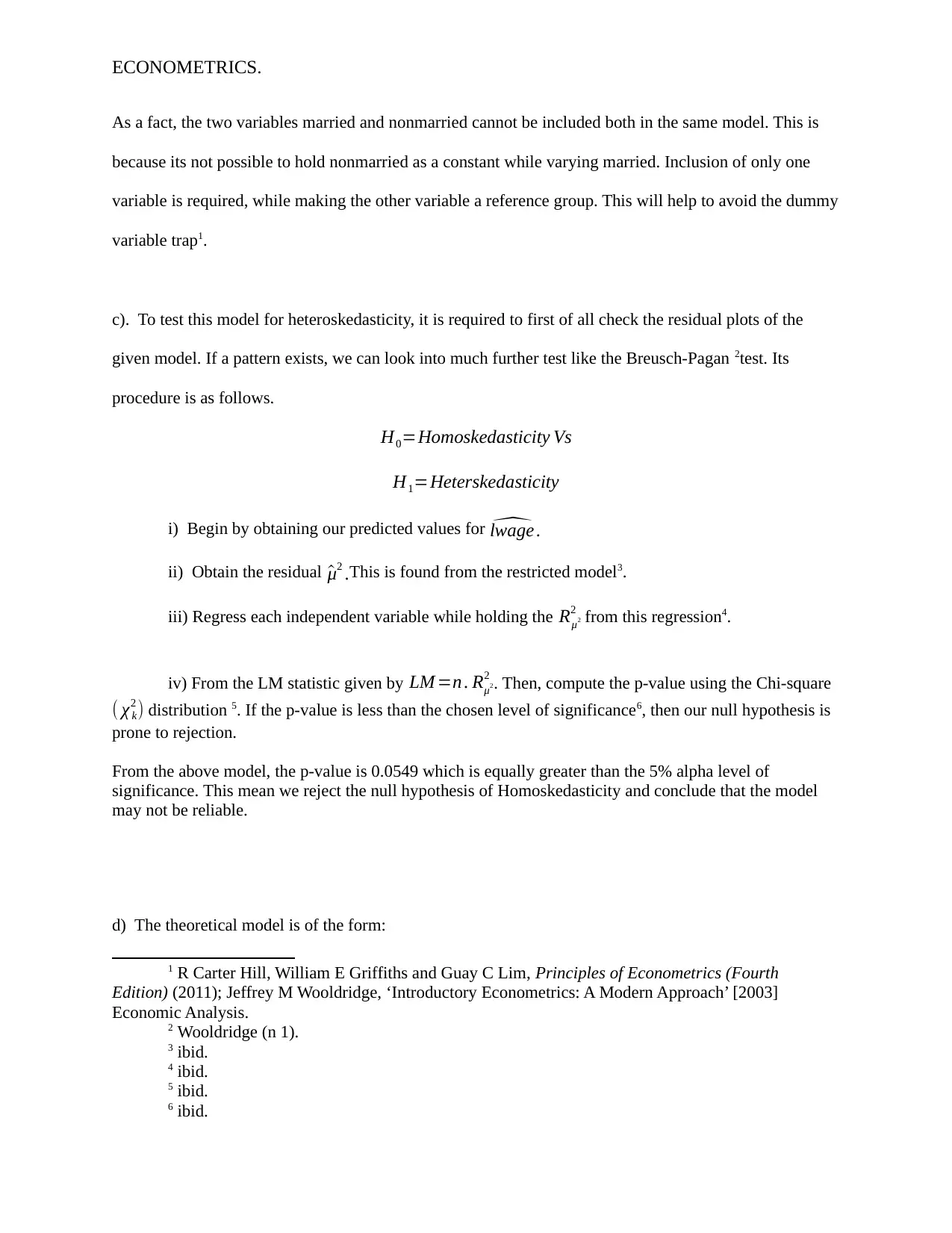
c). To test this model for heteroskedasticity, it is required to first of all check the residual plots of the
given model. If a pattern exists, we can look into much further test like the Breusch-Pagan 2test. Its
procedure is as follows.
H0=Homoskedasticity Vs
H1=Heterskedasticity
i) Begin by obtaining our predicted values for ^lwage .
ii) Obtain the residual ^μ2 .This is found from the restricted model3.
iii) Regress each independent variable while holding the Rμ2
2 from this regression4.
iv) From the LM statistic given by LM =n . Rμ2
2 . Then, compute the p-value using the Chi-square
( χ k
2 ) distribution 5. If the p-value is less than the chosen level of significance6, then our null hypothesis is
prone to rejection.
From the above model, the p-value is 0.0549 which is equally greater than the 5% alpha level of
significance. This mean we reject the null hypothesis of Homoskedasticity and conclude that the model
may not be reliable.
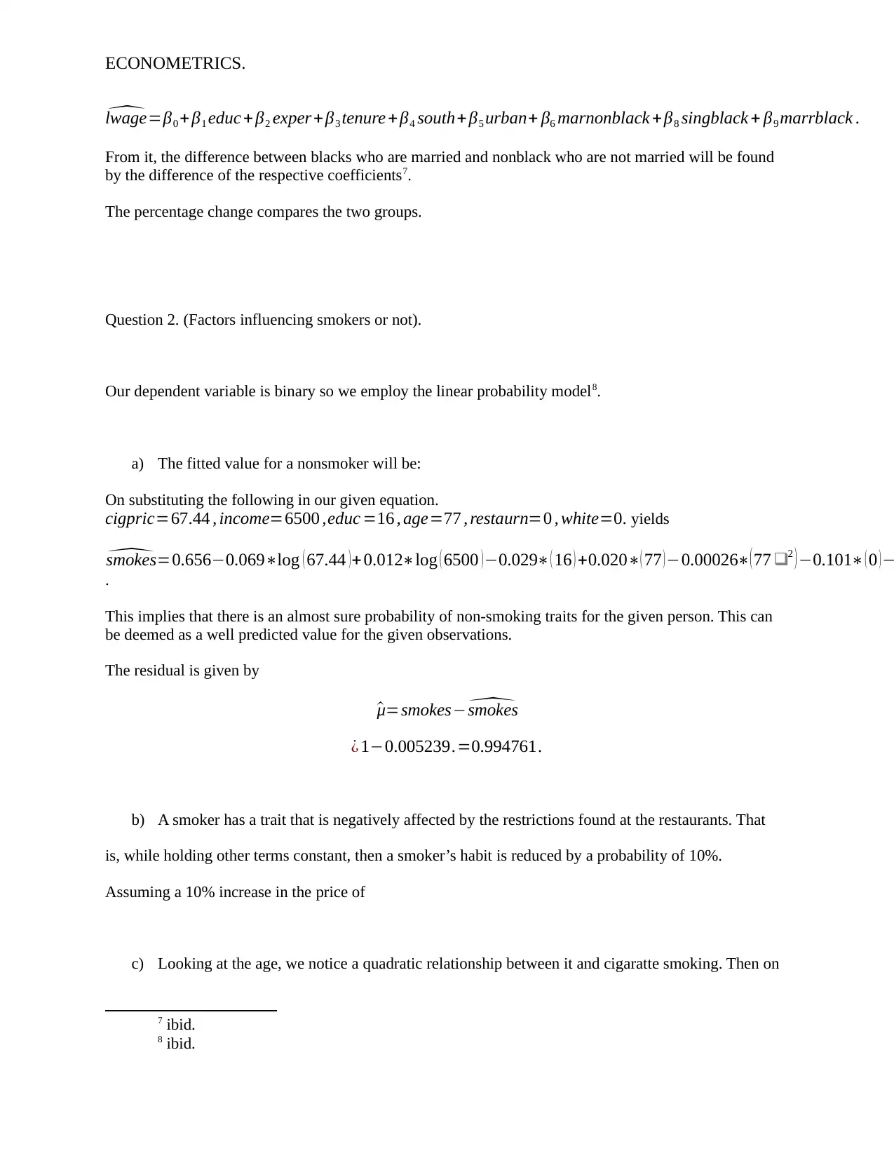
d) The theoretical model is of the form:
1 R Carter Hill, William E Griffiths and Guay C Lim, Principles of Econometrics (Fourth
Edition) (2011); Jeffrey M Wooldridge, ‘Introductory Econometrics: A Modern Approach’ [2003]
Economic Analysis.
2 Wooldridge (n 1).
3 ibid.
4 ibid.
5 ibid.
6 ibid.

ECONOMETRICS.
^lwage=β0 +β1 educ + β2 exper +β3 tenure + β4 south+ β5 urban+ β6 marnonblack + β8 singblack + β9 marrblack .
From it, the difference between blacks who are married and nonblack who are not married will be found
by the difference of the respective coefficients7.
The percentage change compares the two groups.
Question 2. (Factors influencing smokers or not).
Our dependent variable is binary so we employ the linear probability model8.
a) The fitted value for a nonsmoker will be:
On substituting the following in our given equation.
cigpric=67.44 , income=6500 ,educ =16 , age=77 , restaurn=0 , white=0. yields
^smokes=0.656−0.069∗log ( 67.44 )+ 0.012∗log ( 6500 )−0.029∗ ( 16 ) +0.020∗( 77 )−0.00026∗( 77 ❑2 ) −0.101∗ ( 0 )−
.
This implies that there is an almost sure probability of non-smoking traits for the given person. This can
be deemed as a well predicted value for the given observations.
The residual is given by
^μ=smokes− ^smokes
¿ 1−0.005239.=0.994761.
b) A smoker has a trait that is negatively affected by the restrictions found at the restaurants. That
is, while holding other terms constant, then a smoker’s habit is reduced by a probability of 10%.
Assuming a 10% increase in the price of
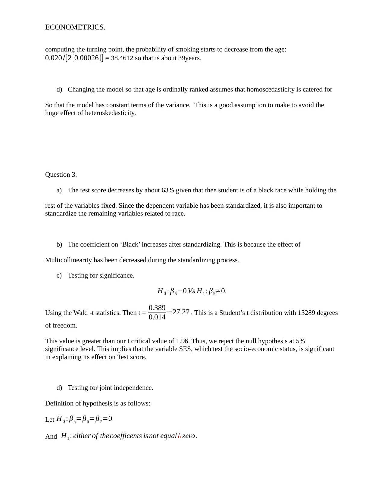
c) Looking at the age, we notice a quadratic relationship between it and cigaratte smoking. Then on
7 ibid.
8 ibid.

ECONOMETRICS.
computing the turning point, the probability of smoking starts to decrease from the age:
0.020 /[2 ( 0.00026 ) ] = 38.4612 so that is about 39years.
d) Changing the model so that age is ordinally ranked assumes that homoscedasticity is catered for
So that the model has constant terms of the variance. This is a good assumption to make to avoid the
huge effect of heteroskedasticity.
Question 3.
a) The test score decreases by about 63% given that thee student is of a black race while holding the
rest of the variables fixed. Since the dependent variable has been standardized, it is also important to
standardize the remaining variables related to race.
b) The coefficient on ‘Black’ increases after standardizing. This is because the effect of
Multicollinearity has been decreased during the standardizing process.
c) Testing for significance.
H0 : β5=0 Vs H1 : β5 ≠ 0.
Using the Wald -t statistics. Then t = 0.389
0.014 =27.27 . This is a Student’s t distribution with 13289 degrees
of freedom.
This value is greater than our t critical value of 1.96. Thus, we reject the null hypothesis at 5%
significance level. This implies that the variable SES, which test the socio-economic status, is significant
in explaining its effect on Test score.
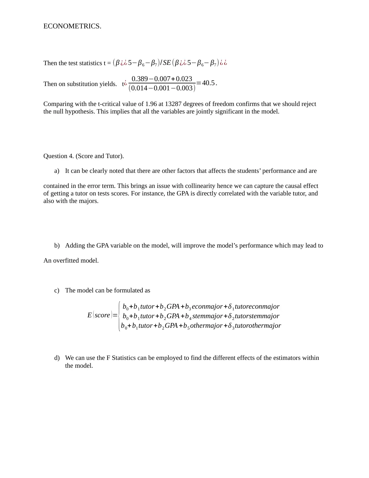
d) Testing for joint independence.
Definition of hypothesis is as follows:
Let H0 : β5=β6=β7=0
And H1 : either of thecoefficents isnot equal¿ zero .

ECONOMETRICS.
Then the test statistics t = (β ¿¿ 5−β6 −β7 )/ SE (β ¿¿ 5−β6− β7 ) ¿ ¿
Then on substitution yields. t¿ 0.389−0.007+ 0.023
(0.014−0.001−0.003)=40.5 .
Comparing with the t-critical value of 1.96 at 13287 degrees of freedom confirms that we should reject
the null hypothesis. This implies that all the variables are jointly significant in the model.
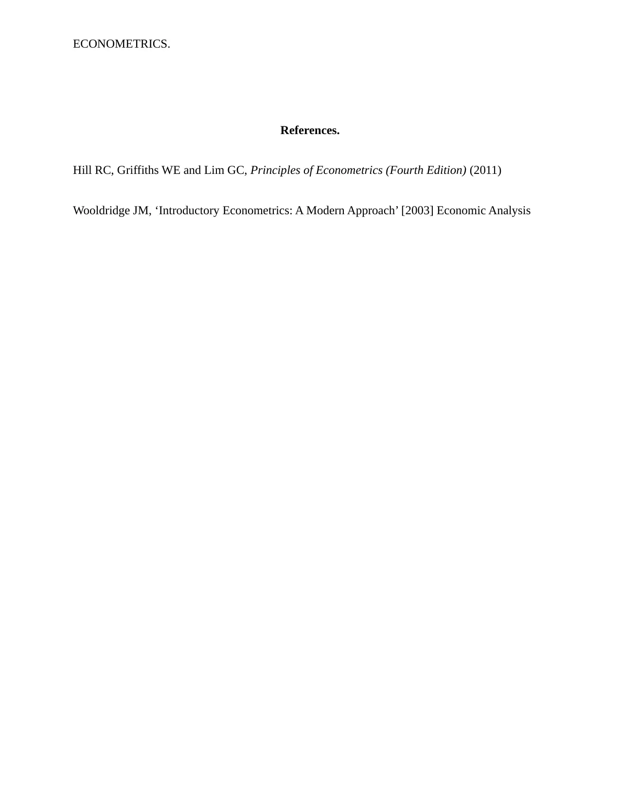
Question 4. (Score and Tutor).
a) It can be clearly noted that there are other factors that affects the students’ performance and are
contained in the error term. This brings an issue with collinearity hence we can capture the causal effect
of getting a tutor on tests scores. For instance, the GPA is directly correlated with the variable tutor, and
also with the majors.
b) Adding the GPA variable on the model, will improve the model’s performance which may lead to
An overfitted model.
c) The model can be formulated as
E ( score ) =
{ b0 +b1 tutor +b2 GPA +b3 econmajor +δ1 tutoreconmajor
b0 +b1 tutor +b2 GPA +b4 stemmajor +δ2 tutorstemmajor
b0+ b1 tutor +b2 GPA +b5 othermajor +δ3 tutorothermajor
d) We can use the F Statistics can be employed to find the different effects of the estimators within
the model.

ECONOMETRICS.
References.
Hill RC, Griffiths WE and Lim GC, Principles of Econometrics (Fourth Edition) (2011)
Wooldridge JM, ‘Introductory Econometrics: A Modern Approach’ [2003] Economic Analysis