Descriptive statistics and histograms
VerifiedAdded on 2023/03/17
|9
|1704
|98
AI Summary
This article provides descriptive statistics and histograms for the variables in the study. It also presents the expected signs for the predictor variables and regression results for estimating the economic model.
Contribute Materials
Your contribution can guide someone’s learning journey. Share your
documents today.

Econometrics
Student Name:
Instructor Name:
Course Number:
8 May 2019
Student Name:
Instructor Name:
Course Number:
8 May 2019
Secure Best Marks with AI Grader
Need help grading? Try our AI Grader for instant feedback on your assignments.
i. Descriptive statistics and histograms
Answer
Descriptive statistics
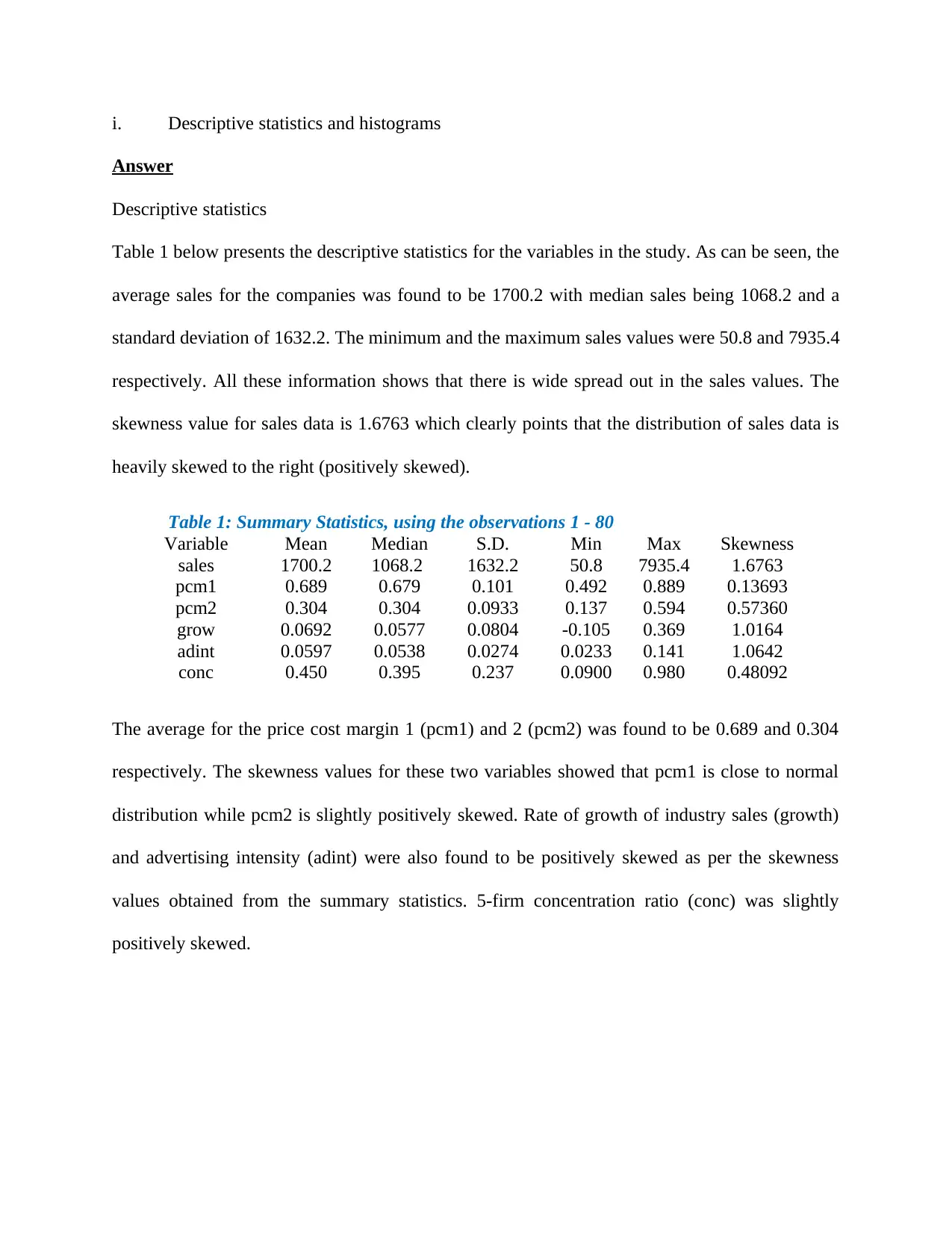
Table 1 below presents the descriptive statistics for the variables in the study. As can be seen, the
average sales for the companies was found to be 1700.2 with median sales being 1068.2 and a
standard deviation of 1632.2. The minimum and the maximum sales values were 50.8 and 7935.4
respectively. All these information shows that there is wide spread out in the sales values. The
skewness value for sales data is 1.6763 which clearly points that the distribution of sales data is
heavily skewed to the right (positively skewed).
Table 1: Summary Statistics, using the observations 1 - 80
Variable Mean Median S.D. Min Max Skewness
sales 1700.2 1068.2 1632.2 50.8 7935.4 1.6763
pcm1 0.689 0.679 0.101 0.492 0.889 0.13693
pcm2 0.304 0.304 0.0933 0.137 0.594 0.57360
grow 0.0692 0.0577 0.0804 -0.105 0.369 1.0164
adint 0.0597 0.0538 0.0274 0.0233 0.141 1.0642
conc 0.450 0.395 0.237 0.0900 0.980 0.48092
The average for the price cost margin 1 (pcm1) and 2 (pcm2) was found to be 0.689 and 0.304
respectively. The skewness values for these two variables showed that pcm1 is close to normal
distribution while pcm2 is slightly positively skewed. Rate of growth of industry sales (growth)
and advertising intensity (adint) were also found to be positively skewed as per the skewness
values obtained from the summary statistics. 5-firm concentration ratio (conc) was slightly
positively skewed.
Answer
Descriptive statistics
Table 1 below presents the descriptive statistics for the variables in the study. As can be seen, the
average sales for the companies was found to be 1700.2 with median sales being 1068.2 and a
standard deviation of 1632.2. The minimum and the maximum sales values were 50.8 and 7935.4
respectively. All these information shows that there is wide spread out in the sales values. The
skewness value for sales data is 1.6763 which clearly points that the distribution of sales data is
heavily skewed to the right (positively skewed).
Table 1: Summary Statistics, using the observations 1 - 80
Variable Mean Median S.D. Min Max Skewness
sales 1700.2 1068.2 1632.2 50.8 7935.4 1.6763
pcm1 0.689 0.679 0.101 0.492 0.889 0.13693
pcm2 0.304 0.304 0.0933 0.137 0.594 0.57360
grow 0.0692 0.0577 0.0804 -0.105 0.369 1.0164
adint 0.0597 0.0538 0.0274 0.0233 0.141 1.0642
conc 0.450 0.395 0.237 0.0900 0.980 0.48092
The average for the price cost margin 1 (pcm1) and 2 (pcm2) was found to be 0.689 and 0.304
respectively. The skewness values for these two variables showed that pcm1 is close to normal
distribution while pcm2 is slightly positively skewed. Rate of growth of industry sales (growth)
and advertising intensity (adint) were also found to be positively skewed as per the skewness
values obtained from the summary statistics. 5-firm concentration ratio (conc) was slightly
positively skewed.
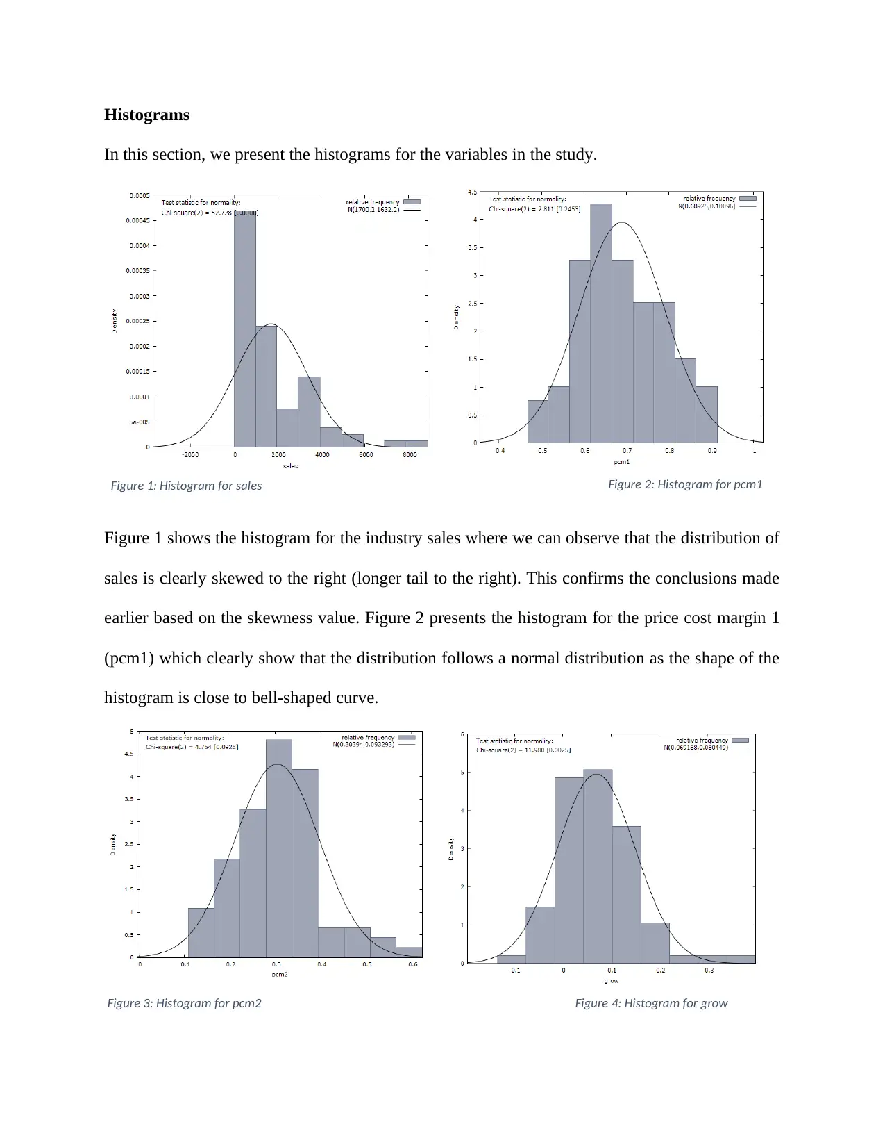
Histograms
In this section, we present the histograms for the variables in the study.
Figure 2: Histogram for pcm1
Figure 1 shows the histogram for the industry sales where we can observe that the distribution of
sales is clearly skewed to the right (longer tail to the right). This confirms the conclusions made
earlier based on the skewness value. Figure 2 presents the histogram for the price cost margin 1
(pcm1) which clearly show that the distribution follows a normal distribution as the shape of the
histogram is close to bell-shaped curve.
Figure 4: Histogram for grow
Figure 1: Histogram for sales
Figure 3: Histogram for pcm2
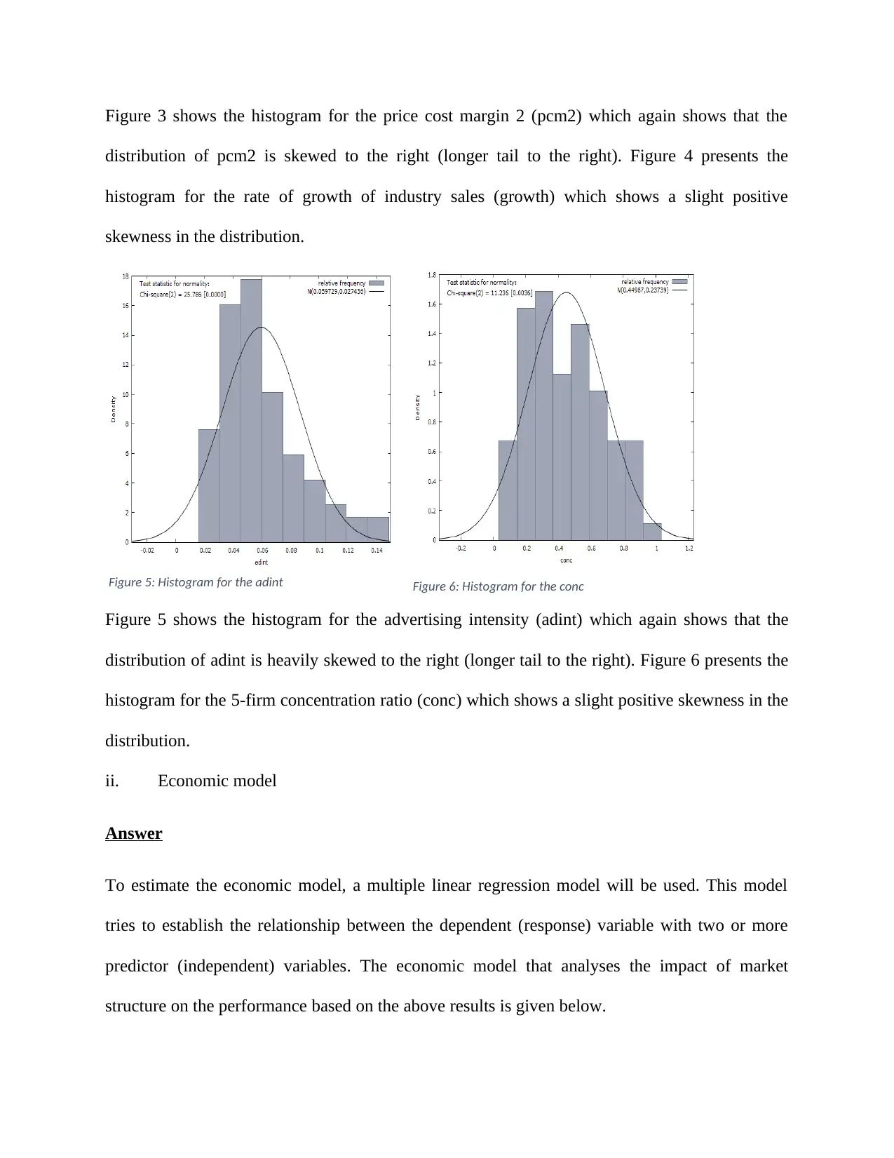
Figure 3 shows the histogram for the price cost margin 2 (pcm2) which again shows that the
distribution of pcm2 is skewed to the right (longer tail to the right). Figure 4 presents the
histogram for the rate of growth of industry sales (growth) which shows a slight positive
skewness in the distribution.
Figure 6: Histogram for the conc
Figure 5 shows the histogram for the advertising intensity (adint) which again shows that the
distribution of adint is heavily skewed to the right (longer tail to the right). Figure 6 presents the
histogram for the 5-firm concentration ratio (conc) which shows a slight positive skewness in the
distribution.
ii. Economic model
Answer
To estimate the economic model, a multiple linear regression model will be used. This model
tries to establish the relationship between the dependent (response) variable with two or more
predictor (independent) variables. The economic model that analyses the impact of market
structure on the performance based on the above results is given below.
Figure 5: Histogram for the adint
Secure Best Marks with AI Grader
Need help grading? Try our AI Grader for instant feedback on your assignments.
y=β0 + β1 x1 + β2 x2 + β3 x3 + β4 x4 + β5 x5 +ε
Where we have the following;
y=industry sales(million GBP)
,
x1=Price cost margin 1, x2=Price cost margin 2 , x3=rate of growth of industry sales , x4 =advertising intensity , x5
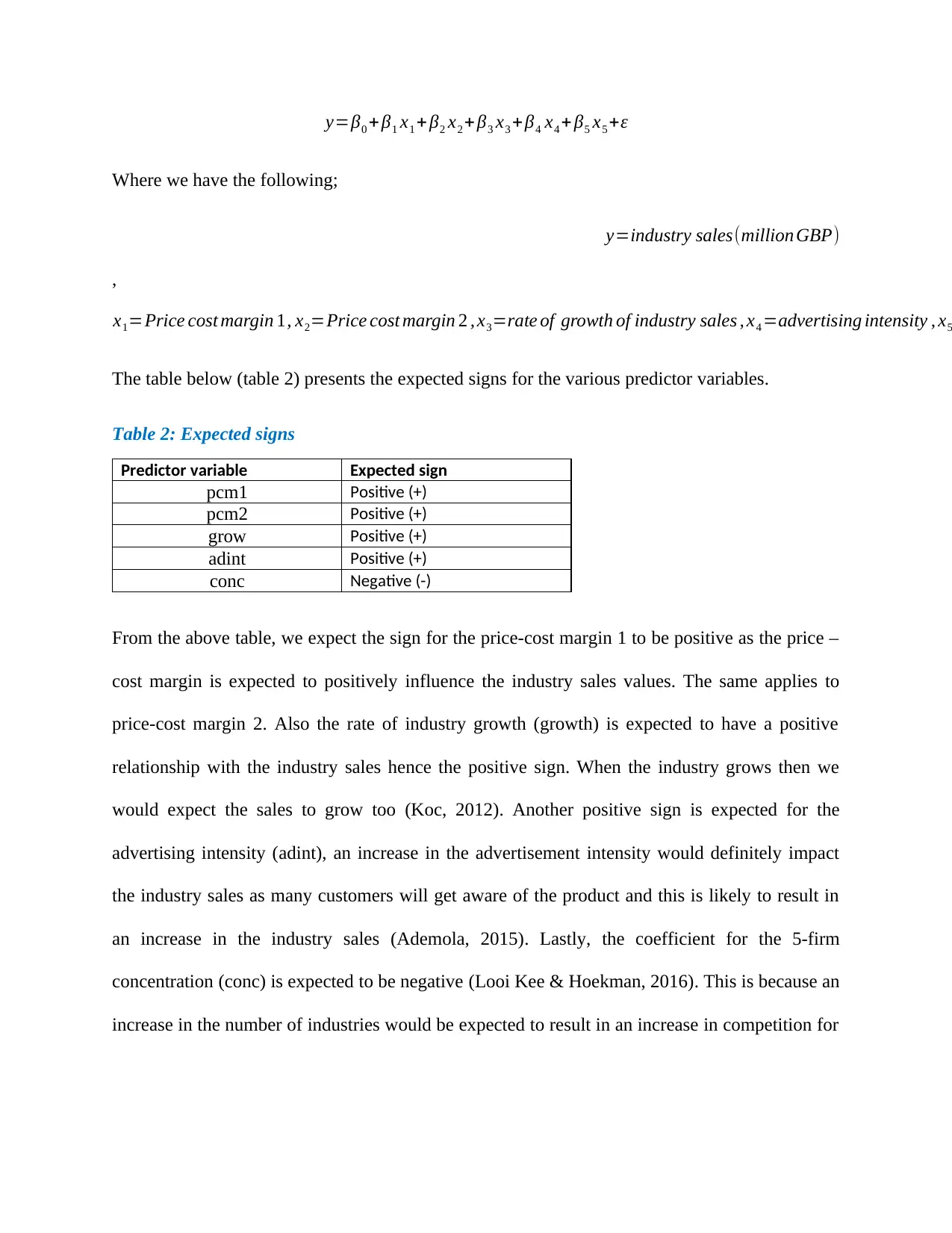
The table below (table 2) presents the expected signs for the various predictor variables.
Table 2: Expected signs
Predictor variable Expected sign
pcm1 Positive (+)
pcm2 Positive (+)
grow Positive (+)
adint Positive (+)
conc Negative (-)
From the above table, we expect the sign for the price-cost margin 1 to be positive as the price –
cost margin is expected to positively influence the industry sales values. The same applies to
price-cost margin 2. Also the rate of industry growth (growth) is expected to have a positive
relationship with the industry sales hence the positive sign. When the industry grows then we
would expect the sales to grow too (Koc, 2012). Another positive sign is expected for the
advertising intensity (adint), an increase in the advertisement intensity would definitely impact
the industry sales as many customers will get aware of the product and this is likely to result in
an increase in the industry sales (Ademola, 2015). Lastly, the coefficient for the 5-firm
concentration (conc) is expected to be negative (Looi Kee & Hoekman, 2016). This is because an
increase in the number of industries would be expected to result in an increase in competition for
Where we have the following;
y=industry sales(million GBP)
,
x1=Price cost margin 1, x2=Price cost margin 2 , x3=rate of growth of industry sales , x4 =advertising intensity , x5
The table below (table 2) presents the expected signs for the various predictor variables.
Table 2: Expected signs
Predictor variable Expected sign
pcm1 Positive (+)
pcm2 Positive (+)
grow Positive (+)
adint Positive (+)
conc Negative (-)
From the above table, we expect the sign for the price-cost margin 1 to be positive as the price –
cost margin is expected to positively influence the industry sales values. The same applies to
price-cost margin 2. Also the rate of industry growth (growth) is expected to have a positive
relationship with the industry sales hence the positive sign. When the industry grows then we
would expect the sales to grow too (Koc, 2012). Another positive sign is expected for the
advertising intensity (adint), an increase in the advertisement intensity would definitely impact
the industry sales as many customers will get aware of the product and this is likely to result in
an increase in the industry sales (Ademola, 2015). Lastly, the coefficient for the 5-firm
concentration (conc) is expected to be negative (Looi Kee & Hoekman, 2016). This is because an
increase in the number of industries would be expected to result in an increase in competition for
the available customers hence leading to a reduction in the industry sales for a company
(McCloughan, et al., 2012).
iii. Estimated econometric model
Answer
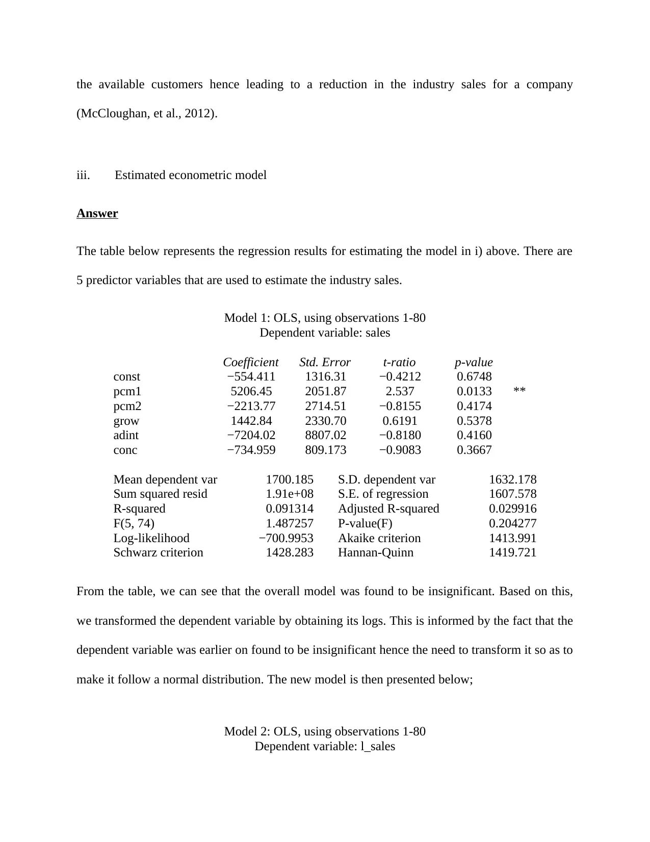
The table below represents the regression results for estimating the model in i) above. There are
5 predictor variables that are used to estimate the industry sales.
Model 1: OLS, using observations 1-80
Dependent variable: sales
Coefficient Std. Error t-ratio p-value
const −554.411 1316.31 −0.4212 0.6748
pcm1 5206.45 2051.87 2.537 0.0133 **
pcm2 −2213.77 2714.51 −0.8155 0.4174
grow 1442.84 2330.70 0.6191 0.5378
adint −7204.02 8807.02 −0.8180 0.4160
conc −734.959 809.173 −0.9083 0.3667
Mean dependent var 1700.185 S.D. dependent var 1632.178
Sum squared resid 1.91e+08 S.E. of regression 1607.578
R-squared 0.091314 Adjusted R-squared 0.029916
F(5, 74) 1.487257 P-value(F) 0.204277
Log-likelihood −700.9953 Akaike criterion 1413.991
Schwarz criterion 1428.283 Hannan-Quinn 1419.721
From the table, we can see that the overall model was found to be insignificant. Based on this,
we transformed the dependent variable by obtaining its logs. This is informed by the fact that the
dependent variable was earlier on found to be insignificant hence the need to transform it so as to
make it follow a normal distribution. The new model is then presented below;
Model 2: OLS, using observations 1-80
Dependent variable: l_sales
(McCloughan, et al., 2012).
iii. Estimated econometric model
Answer
The table below represents the regression results for estimating the model in i) above. There are
5 predictor variables that are used to estimate the industry sales.
Model 1: OLS, using observations 1-80
Dependent variable: sales
Coefficient Std. Error t-ratio p-value
const −554.411 1316.31 −0.4212 0.6748
pcm1 5206.45 2051.87 2.537 0.0133 **
pcm2 −2213.77 2714.51 −0.8155 0.4174
grow 1442.84 2330.70 0.6191 0.5378
adint −7204.02 8807.02 −0.8180 0.4160
conc −734.959 809.173 −0.9083 0.3667
Mean dependent var 1700.185 S.D. dependent var 1632.178
Sum squared resid 1.91e+08 S.E. of regression 1607.578
R-squared 0.091314 Adjusted R-squared 0.029916
F(5, 74) 1.487257 P-value(F) 0.204277
Log-likelihood −700.9953 Akaike criterion 1413.991
Schwarz criterion 1428.283 Hannan-Quinn 1419.721
From the table, we can see that the overall model was found to be insignificant. Based on this,
we transformed the dependent variable by obtaining its logs. This is informed by the fact that the
dependent variable was earlier on found to be insignificant hence the need to transform it so as to
make it follow a normal distribution. The new model is then presented below;
Model 2: OLS, using observations 1-80
Dependent variable: l_sales
Coefficient Std. Error t-ratio p-value
const 4.53617 0.868398 5.224 <0.0001 ***
pcm1 5.28225 1.35366 3.902 0.0002 ***
pcm2 −1.33369 1.79083 −0.7447 0.4588
grow −0.0777298 1.53762 −0.05055 0.9598
adint −6.61067 5.81020 −1.138 0.2589
conc −0.970111 0.533830 −1.817 0.0732 *
Mean dependent var 6.934951 S.D. dependent var 1.139659
Sum squared resid 83.23375 S.E. of regression 1.060557
R-squared 0.188811 Adjusted R-squared 0.134000
F(5, 74) 3.444814 P-value(F) 0.007468
Log-likelihood −115.1001 Akaike criterion 242.2003
Schwarz criterion 256.4924 Hannan-Quinn 247.9304
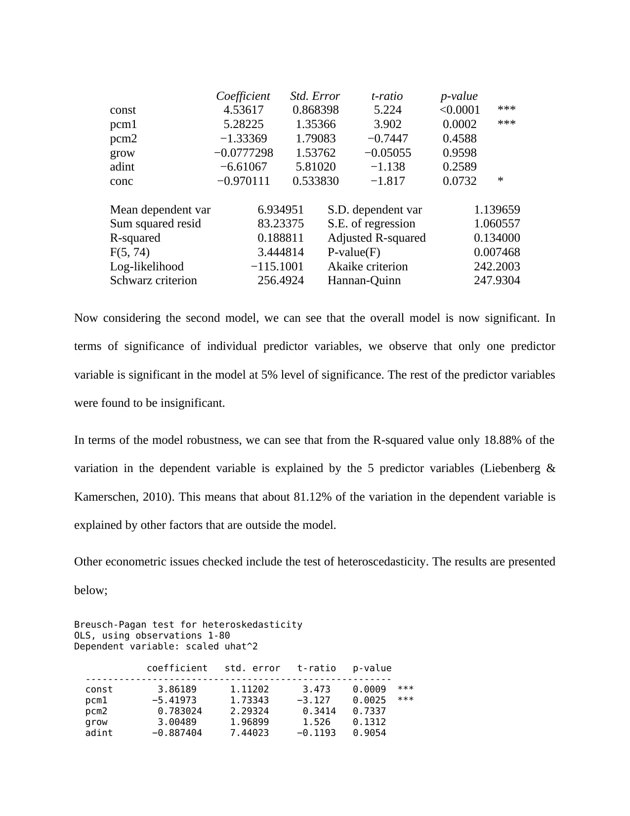
Now considering the second model, we can see that the overall model is now significant. In
terms of significance of individual predictor variables, we observe that only one predictor
variable is significant in the model at 5% level of significance. The rest of the predictor variables
were found to be insignificant.
In terms of the model robustness, we can see that from the R-squared value only 18.88% of the
variation in the dependent variable is explained by the 5 predictor variables (Liebenberg &
Kamerschen, 2010). This means that about 81.12% of the variation in the dependent variable is
explained by other factors that are outside the model.
Other econometric issues checked include the test of heteroscedasticity. The results are presented
below;
Breusch-Pagan test for heteroskedasticity
OLS, using observations 1-80
Dependent variable: scaled uhat^2
coefficient std. error t-ratio p-value
-------------------------------------------------------
const 3.86189 1.11202 3.473 0.0009 ***
pcm1 −5.41973 1.73343 −3.127 0.0025 ***
pcm2 0.783024 2.29324 0.3414 0.7337
grow 3.00489 1.96899 1.526 0.1312
adint −0.887404 7.44023 −0.1193 0.9054
const 4.53617 0.868398 5.224 <0.0001 ***
pcm1 5.28225 1.35366 3.902 0.0002 ***
pcm2 −1.33369 1.79083 −0.7447 0.4588
grow −0.0777298 1.53762 −0.05055 0.9598
adint −6.61067 5.81020 −1.138 0.2589
conc −0.970111 0.533830 −1.817 0.0732 *
Mean dependent var 6.934951 S.D. dependent var 1.139659
Sum squared resid 83.23375 S.E. of regression 1.060557
R-squared 0.188811 Adjusted R-squared 0.134000
F(5, 74) 3.444814 P-value(F) 0.007468
Log-likelihood −115.1001 Akaike criterion 242.2003
Schwarz criterion 256.4924 Hannan-Quinn 247.9304
Now considering the second model, we can see that the overall model is now significant. In
terms of significance of individual predictor variables, we observe that only one predictor
variable is significant in the model at 5% level of significance. The rest of the predictor variables
were found to be insignificant.
In terms of the model robustness, we can see that from the R-squared value only 18.88% of the
variation in the dependent variable is explained by the 5 predictor variables (Liebenberg &
Kamerschen, 2010). This means that about 81.12% of the variation in the dependent variable is
explained by other factors that are outside the model.
Other econometric issues checked include the test of heteroscedasticity. The results are presented
below;
Breusch-Pagan test for heteroskedasticity
OLS, using observations 1-80
Dependent variable: scaled uhat^2
coefficient std. error t-ratio p-value
-------------------------------------------------------
const 3.86189 1.11202 3.473 0.0009 ***
pcm1 −5.41973 1.73343 −3.127 0.0025 ***
pcm2 0.783024 2.29324 0.3414 0.7337
grow 3.00489 1.96899 1.526 0.1312
adint −0.887404 7.44023 −0.1193 0.9054
Paraphrase This Document
Need a fresh take? Get an instant paraphrase of this document with our AI Paraphraser
conc 1.06867 0.683595 1.563 0.1222
Explained sum of squares = 30.2084
Test statistic: LM = 15.104176,
with p-value = P(Chi-square(5) > 15.104176) = 0.009926
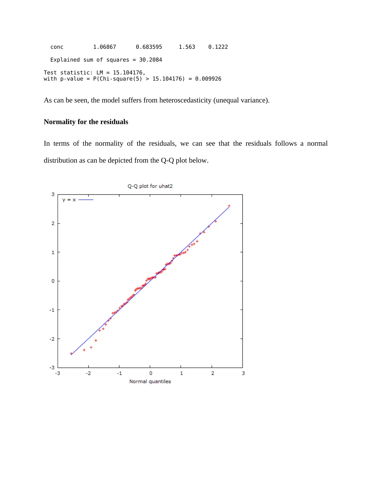
As can be seen, the model suffers from heteroscedasticity (unequal variance).
Normality for the residuals
In terms of the normality of the residuals, we can see that the residuals follows a normal
distribution as can be depicted from the Q-Q plot below.
Explained sum of squares = 30.2084
Test statistic: LM = 15.104176,
with p-value = P(Chi-square(5) > 15.104176) = 0.009926
As can be seen, the model suffers from heteroscedasticity (unequal variance).
Normality for the residuals
In terms of the normality of the residuals, we can see that the residuals follows a normal
distribution as can be depicted from the Q-Q plot below.

References
Ademola, O., 2015. Effects of Gender-Role Orientation, Sex of Advert Presenter and Product
Type on Advertising Effectiveness. European Journal of Scientific Research, 35(4), p. 537–543.
Koc, E., 2012. Impact of gender in marketing communications: the role of cognitive and
affective cues. Journal of Marketing Communications, 8(4), p. 257.
Liebenberg, A. P. & Kamerschen, D. R., 2010. Structure, conduct, and performance analysis of
the south African auto insurance market: 1980-2000. South African Journal of Economics, 76(2),
pp. 228-238.
Looi Kee, H. & Hoekman, B., 2016. Imports, entry, and competition law as market disciplines.
European Economic Review, 51(4), pp. 831-858.
McCloughan, H. et al., 2012. The effectiveness of competition policy and the price-cost margin:
evidence from panel data. Working Paper No. 209, 32(5), pp. 56-71.
1 out of 9
Related Documents


Your All-in-One AI-Powered Toolkit for Academic Success.
+13062052269
info@desklib.com
Available 24*7 on WhatsApp / Email
![[object Object]](/_next/static/media/star-bottom.7253800d.svg)
Unlock your academic potential
© 2024 | Zucol Services PVT LTD | All rights reserved.