Financial Decision Analysis with Statistics
VerifiedAdded on 2022/11/26
|13
|2468
|364
AI Summary
This document explores the use of statistical data analysis techniques in financial decision making. It discusses the relationship between market prices and variables such as land size, age of the house, and price index. The document includes scatter diagrams, regression models, significance of coefficients, and estimated market prices. The analysis is based on a sample size of 15 and uses the OLS technique.
Contribute Materials
Your contribution can guide someone’s learning journey. Share your
documents today.

Running head: FINANCIAL DECISION ANALYSIS WITH STATISTICS
Financial Decision Analysis with Statistics
Name of the Student:
Name of the University:
Author Note:
Financial Decision Analysis with Statistics
Name of the Student:
Name of the University:
Author Note:
Secure Best Marks with AI Grader
Need help grading? Try our AI Grader for instant feedback on your assignments.
1FINANCIAL DECISION ANALYSIS WITH STATISTICS
Table of Contents
1. Introduction........................................................................................................................2
2. Scatter Diagrams................................................................................................................2
3. First Regression Model......................................................................................................5
4. Regression Equation and Interpretation.............................................................................6
5. Significance of the Estimated Coefficients........................................................................7
6. Coefficient of Determination (Adjusted R2)......................................................................8
7. 95% Confidence Interval of Parameters............................................................................8
8. Second Regression Model..................................................................................................9
9. Comparison between Two Models...................................................................................10
10. Estimated Market Price of House.................................................................................10
Reference..................................................................................................................................11
2FINANCIAL DECISION ANALYSIS WITH STATISTICS
1. Introduction
The financial decisions can be made with the help of statistical data analysis
techniques. This is used to predict the future market price or other market conditions (Vogel
2018). Here, the analysis wants to find the relation between market price of houses with land
size of the area, age of the house and the price index for which a data set is available on the
above mentioned variables. The data is available from 2002-3 to 2016-17 and thus the sample
size of the data is 15. In this case the dependent variable is the market rice of house and the
other variables are the independent variables that may have the influence on the dependent
variable (Brooks 2019). To check the influence, a linear model is formed that will be
analyzed by the OLS technique (McCullagh 2018). The linear model is presented below:
market price=β0+(β ¿¿ 1∗Sydney price Index)+ ( β2∗annual percent change ) + ( β3∗total number of square met
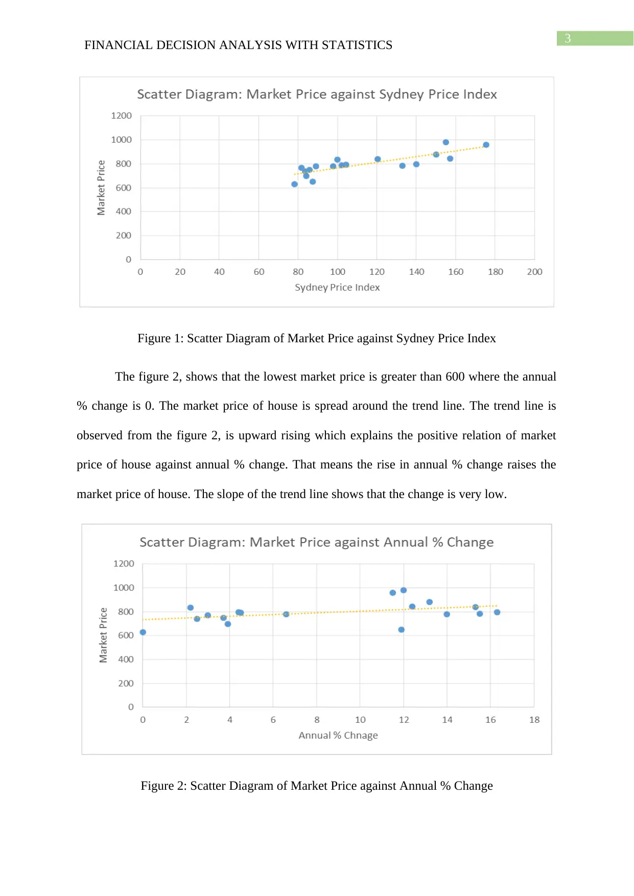
2. Scatter Diagrams
The figure 1, shows that the lowest market price is greater than 600 where the Sydney
Price Index is 80. After the index value 80, market price of house rises. The trend line is
observed from the figure 1, is upward rising which explains the positive relation of market
price of house against Sydney Price Index. That means the rise in Sydney Price Index raises
the market price of house.
1. Introduction
The financial decisions can be made with the help of statistical data analysis
techniques. This is used to predict the future market price or other market conditions (Vogel
2018). Here, the analysis wants to find the relation between market price of houses with land
size of the area, age of the house and the price index for which a data set is available on the
above mentioned variables. The data is available from 2002-3 to 2016-17 and thus the sample
size of the data is 15. In this case the dependent variable is the market rice of house and the
other variables are the independent variables that may have the influence on the dependent
variable (Brooks 2019). To check the influence, a linear model is formed that will be
analyzed by the OLS technique (McCullagh 2018). The linear model is presented below:
market price=β0+(β ¿¿ 1∗Sydney price Index)+ ( β2∗annual percent change ) + ( β3∗total number of square met
2. Scatter Diagrams
The figure 1, shows that the lowest market price is greater than 600 where the Sydney
Price Index is 80. After the index value 80, market price of house rises. The trend line is
observed from the figure 1, is upward rising which explains the positive relation of market
price of house against Sydney Price Index. That means the rise in Sydney Price Index raises
the market price of house.
3FINANCIAL DECISION ANALYSIS WITH STATISTICS
Figure 1: Scatter Diagram of Market Price against Sydney Price Index
The figure 2, shows that the lowest market price is greater than 600 where the annual
% change is 0. The market price of house is spread around the trend line. The trend line is
observed from the figure 2, is upward rising which explains the positive relation of market
price of house against annual % change. That means the rise in annual % change raises the
market price of house. The slope of the trend line shows that the change is very low.
Figure 2: Scatter Diagram of Market Price against Annual % Change
Secure Best Marks with AI Grader
Need help grading? Try our AI Grader for instant feedback on your assignments.
4FINANCIAL DECISION ANALYSIS WITH STATISTICS
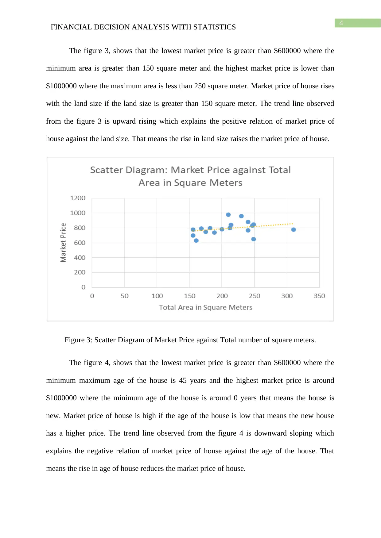
The figure 3, shows that the lowest market price is greater than $600000 where the
minimum area is greater than 150 square meter and the highest market price is lower than
$1000000 where the maximum area is less than 250 square meter. Market price of house rises
with the land size if the land size is greater than 150 square meter. The trend line observed
from the figure 3 is upward rising which explains the positive relation of market price of
house against the land size. That means the rise in land size raises the market price of house.
Figure 3: Scatter Diagram of Market Price against Total number of square meters.
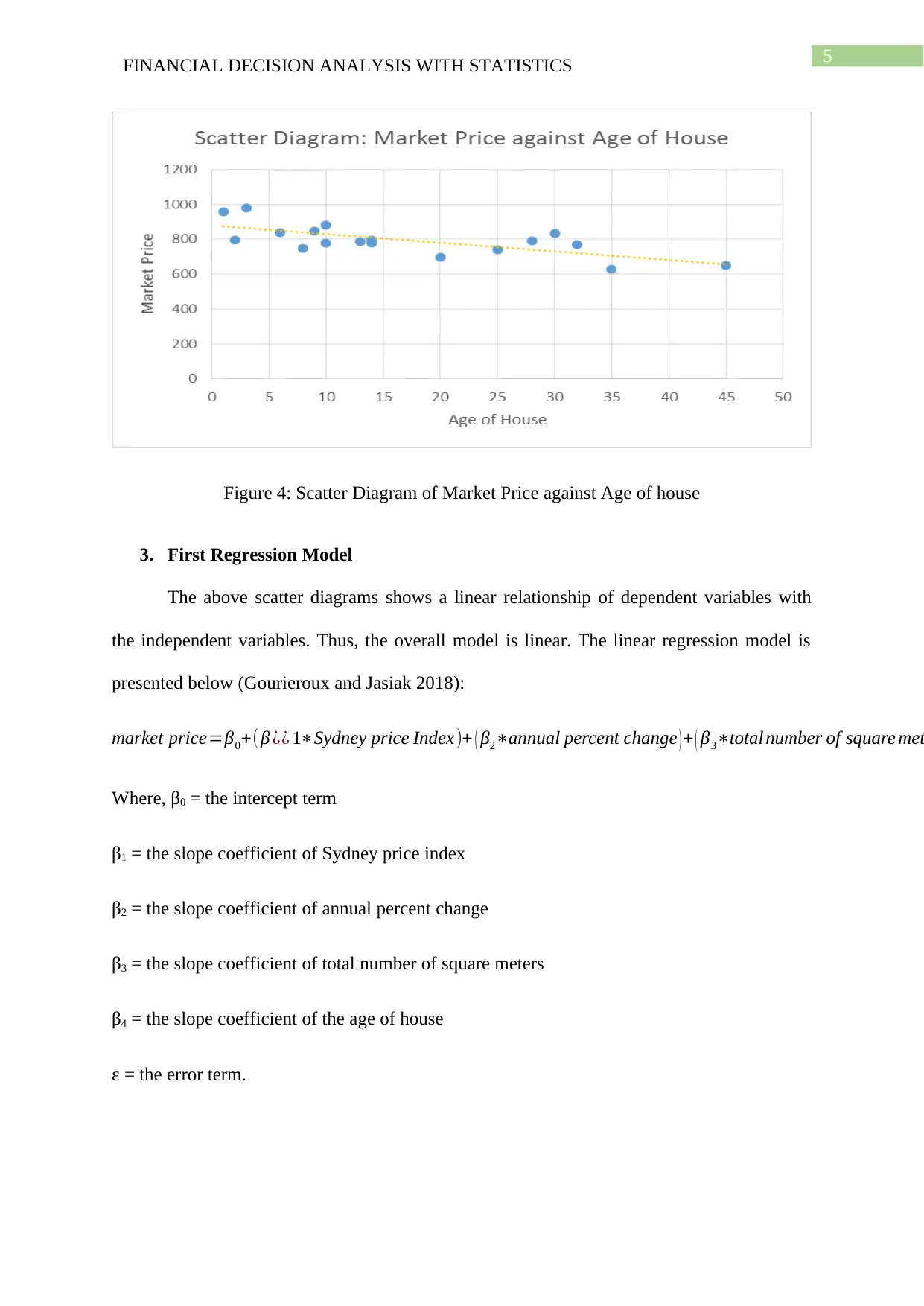
The figure 4, shows that the lowest market price is greater than $600000 where the
minimum maximum age of the house is 45 years and the highest market price is around
$1000000 where the minimum age of the house is around 0 years that means the house is
new. Market price of house is high if the age of the house is low that means the new house
has a higher price. The trend line observed from the figure 4 is downward sloping which
explains the negative relation of market price of house against the age of the house. That
means the rise in age of house reduces the market price of house.
The figure 3, shows that the lowest market price is greater than $600000 where the
minimum area is greater than 150 square meter and the highest market price is lower than
$1000000 where the maximum area is less than 250 square meter. Market price of house rises
with the land size if the land size is greater than 150 square meter. The trend line observed
from the figure 3 is upward rising which explains the positive relation of market price of
house against the land size. That means the rise in land size raises the market price of house.
Figure 3: Scatter Diagram of Market Price against Total number of square meters.
The figure 4, shows that the lowest market price is greater than $600000 where the
minimum maximum age of the house is 45 years and the highest market price is around
$1000000 where the minimum age of the house is around 0 years that means the house is
new. Market price of house is high if the age of the house is low that means the new house
has a higher price. The trend line observed from the figure 4 is downward sloping which
explains the negative relation of market price of house against the age of the house. That
means the rise in age of house reduces the market price of house.
5FINANCIAL DECISION ANALYSIS WITH STATISTICS
Figure 4: Scatter Diagram of Market Price against Age of house
3. First Regression Model
The above scatter diagrams shows a linear relationship of dependent variables with
the independent variables. Thus, the overall model is linear. The linear regression model is
presented below (Gourieroux and Jasiak 2018):
market price=β0+(β ¿¿ 1∗Sydney price Index)+ ( β2∗annual percent change ) + ( β3∗total number of square met
Where, β0 = the intercept term
β1 = the slope coefficient of Sydney price index
β2 = the slope coefficient of annual percent change
β3 = the slope coefficient of total number of square meters
β4 = the slope coefficient of the age of house
ε = the error term.
6FINANCIAL DECISION ANALYSIS WITH STATISTICS
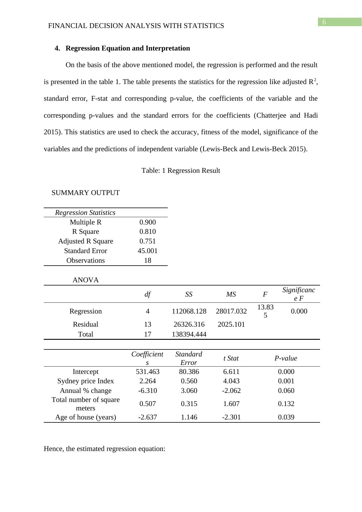
4. Regression Equation and Interpretation
On the basis of the above mentioned model, the regression is performed and the result
is presented in the table 1. The table presents the statistics for the regression like adjusted R2,
standard error, F-stat and corresponding p-value, the coefficients of the variable and the
corresponding p-values and the standard errors for the coefficients (Chatterjee and Hadi
2015). This statistics are used to check the accuracy, fitness of the model, significance of the
variables and the predictions of independent variable (Lewis-Beck and Lewis-Beck 2015).
Table: 1 Regression Result
SUMMARY OUTPUT
Regression Statistics
Multiple R 0.900
R Square 0.810
Adjusted R Square 0.751
Standard Error 45.001
Observations 18
ANOVA
df SS MS F Significanc
e F
Regression 4 112068.128 28017.032 13.83
5 0.000
Residual 13 26326.316 2025.101
Total 17 138394.444
Coefficient
s
Standard
Error t Stat P-value
Intercept 531.463 80.386 6.611 0.000
Sydney price Index 2.264 0.560 4.043 0.001
Annual % change -6.310 3.060 -2.062 0.060
Total number of square
meters 0.507 0.315 1.607 0.132
Age of house (years) -2.637 1.146 -2.301 0.039
Hence, the estimated regression equation:
Paraphrase This Document
Need a fresh take? Get an instant paraphrase of this document with our AI Paraphraser
7FINANCIAL DECISION ANALYSIS WITH STATISTICS
^market price=548.978+ ( 2.264∗Sydney price Index ) − ( 6.310∗annual percent change ) + ( 0.507∗total number o
Where, ^market price= the estimated market price.
5. Significance of the Estimated Coefficients
The estimated coefficient from the regression that are presented in the table 1
indicates the amount of change in the market price of house. The coefficients of the
independent variable are nothing but the amount of change in the dependent variable due to
one unit change in the independent variable. However, to interpret the coefficient it is
necessary to check the significance of the coefficients with the help of given corresponding p-
values. The interpretation of each coefficient is discussed below:
β1 = 2.264 is the slope coefficient of Sydney price index. The amount of change in market
price of house is $(2.264*1000) = $2264 due to one unit change in the Sydney Price Index.
The positive value of the coefficient indicates the positive relation. The corresponding p-
value is 0.001 which is less than 0.05 that indicates 5% significance level of the variable (Lee
2016). Now, it can be interpreted as one unit rise in the Sydney Price Index raises the market
price of house by $2264 at 5% significance level.
β2= -6.310 is the slope coefficient of annual % change. The amount of change in market
price of house is $6.310*1000) = $6310 due to one unit change in the annual % change. The
negative value of the coefficient indicates the negative relation. The corresponding p-value is
0.060 which is greater than 0.05 that indicates the variable is not significant at 5%
significance level. Now, it can be interpreted as there is no change in market price due to any
change in the annual % change (Aydin and Malcioglu 2016).
β3 = 0.507 is the slope coefficient of total number of square meters that is land size. The
amount of change in market price of house is $(0.507*1000) = $5070 due to one unit change
in the land size. The positive value of the coefficient indicates the positive relation. The
8FINANCIAL DECISION ANALYSIS WITH STATISTICS
corresponding p-value is 0.132 which is greater than 0.05 that indicates the variable is not
significant at 5% significance level of the variable. Now, it can be interpreted as there is no
change in market price of house due to any change in the land size.
β4 = -2.637 is the slope coefficient of age of house. The amount of change in market price of
house is $(2.637*1000) = $2637 due to one unit change in the age of house. The negative
value of the coefficient indicates the negative relation. The corresponding p-value is 0.039
which is less than 0.05 that indicates 5% significance level of the variable. Now, it can be
interpreted as one unit rise in the age of house reduces the market price of house by $2637 at
5% significance level (Fumo and Biswas 2015.).
6. Coefficient of Determination (Adjusted R2)
Coefficient of determination is nothing but the adjusted R2 for a multivariate linear
regression analysis. This measures the variance in the dependent variable with the help of
independent variables. If the adjusted R2 is equal to 1 then it can be said that there is no error
in the dependent variable and implies a perfect explanation of dependent variable through the
independent variables (Schober, Boer and Schwarte 2018). The adjusted R2 for the above
mentioned model is 0.751 which implies that the market price of house can be predicted by
independent variables through the model at 75.1% accuracy (Austin and Steyerberg 2015).
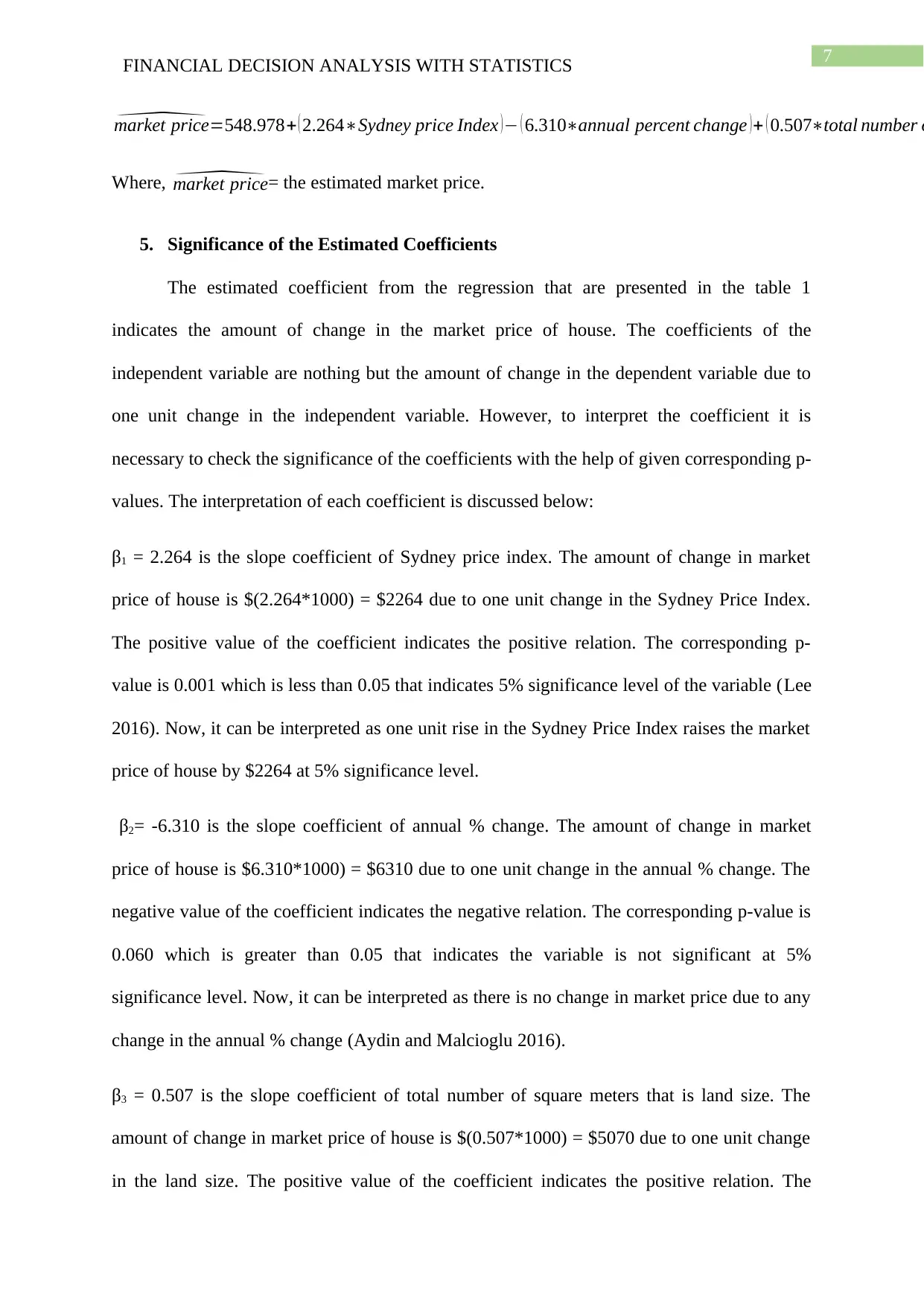
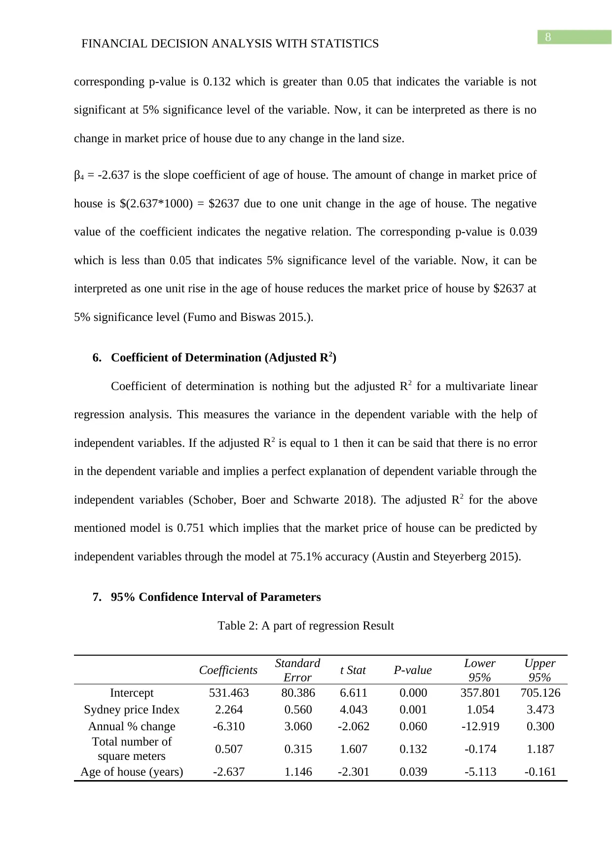
7. 95% Confidence Interval of Parameters
Table 2: A part of regression Result
Coefficients Standard
Error t Stat P-value Lower
95%
Upper
95%
Intercept 531.463 80.386 6.611 0.000 357.801 705.126
Sydney price Index 2.264 0.560 4.043 0.001 1.054 3.473
Annual % change -6.310 3.060 -2.062 0.060 -12.919 0.300
Total number of
square meters 0.507 0.315 1.607 0.132 -0.174 1.187
Age of house (years) -2.637 1.146 -2.301 0.039 -5.113 -0.161
corresponding p-value is 0.132 which is greater than 0.05 that indicates the variable is not
significant at 5% significance level of the variable. Now, it can be interpreted as there is no
change in market price of house due to any change in the land size.
β4 = -2.637 is the slope coefficient of age of house. The amount of change in market price of
house is $(2.637*1000) = $2637 due to one unit change in the age of house. The negative
value of the coefficient indicates the negative relation. The corresponding p-value is 0.039
which is less than 0.05 that indicates 5% significance level of the variable. Now, it can be
interpreted as one unit rise in the age of house reduces the market price of house by $2637 at
5% significance level (Fumo and Biswas 2015.).
6. Coefficient of Determination (Adjusted R2)
Coefficient of determination is nothing but the adjusted R2 for a multivariate linear
regression analysis. This measures the variance in the dependent variable with the help of
independent variables. If the adjusted R2 is equal to 1 then it can be said that there is no error
in the dependent variable and implies a perfect explanation of dependent variable through the
independent variables (Schober, Boer and Schwarte 2018). The adjusted R2 for the above
mentioned model is 0.751 which implies that the market price of house can be predicted by
independent variables through the model at 75.1% accuracy (Austin and Steyerberg 2015).
7. 95% Confidence Interval of Parameters
Table 2: A part of regression Result
Coefficients Standard
Error t Stat P-value Lower
95%
Upper
95%
Intercept 531.463 80.386 6.611 0.000 357.801 705.126
Sydney price Index 2.264 0.560 4.043 0.001 1.054 3.473
Annual % change -6.310 3.060 -2.062 0.060 -12.919 0.300
Total number of
square meters 0.507 0.315 1.607 0.132 -0.174 1.187
Age of house (years) -2.637 1.146 -2.301 0.039 -5.113 -0.161
9FINANCIAL DECISION ANALYSIS WITH STATISTICS
The 95% confidence interval presents a range. Within the range, population mean lies
with 95% certainty.
1.054 ≤ β1 ≥ 3.473, indicates that the coefficient exists between 1.054 and 3.473 at 95%
certainty.
-12.919≤ β2 ≥ 0.300, indicates that the coefficient exists between -12.919 and 0.300 at 95%
certainty.
-0.174 ≤ β3 ≥ 1.187, indicates that the coefficient exists between -0.174 and 1.187 at 95%
certainty.
-5.113≤ β4 ≥ -0.161, indicates that the coefficient exists between -5.113 and -0.161 at 95%
certainty.
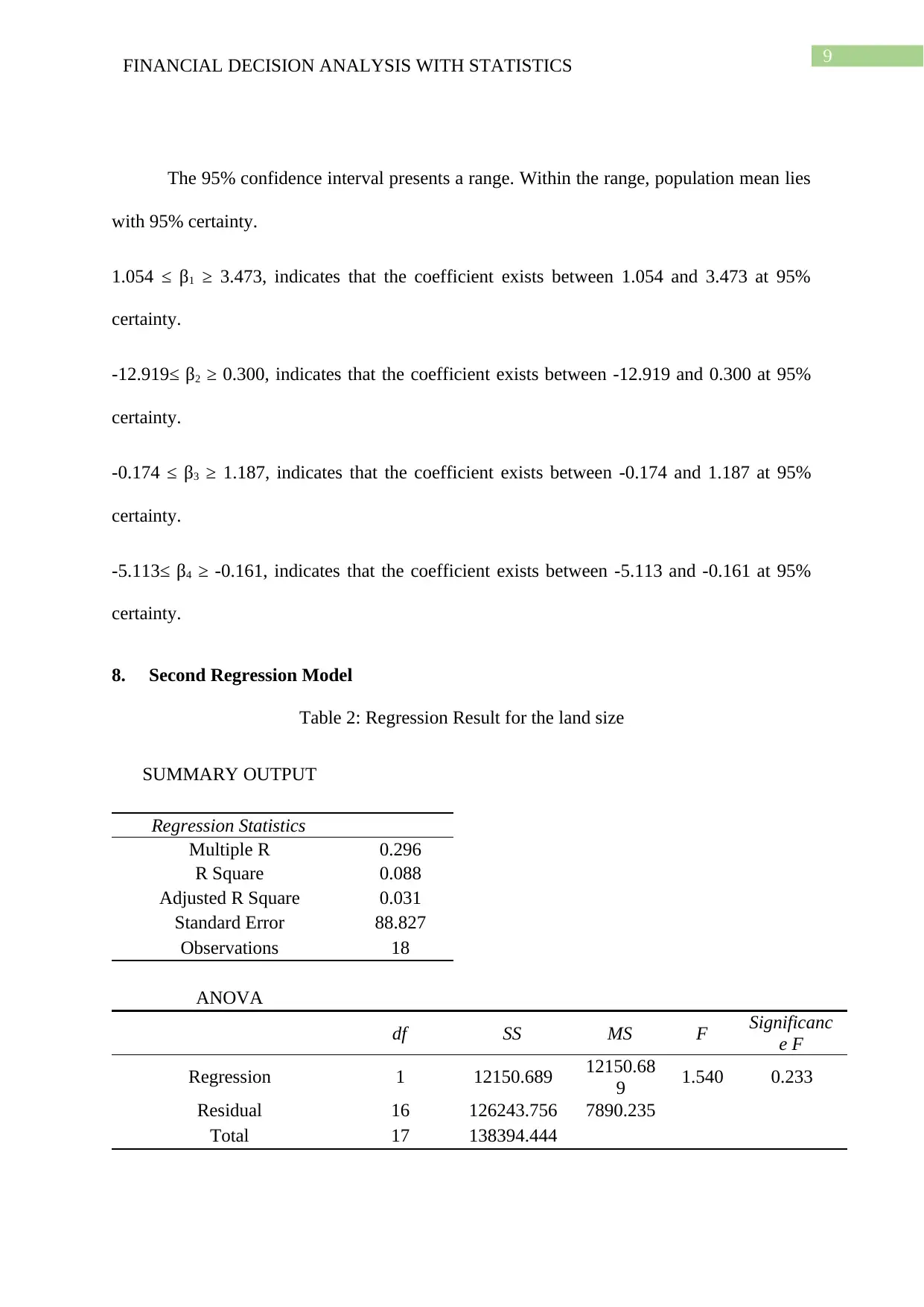
8. Second Regression Model
Table 2: Regression Result for the land size
SUMMARY OUTPUT
Regression Statistics
Multiple R 0.296
R Square 0.088
Adjusted R Square 0.031
Standard Error 88.827
Observations 18
ANOVA
df SS MS F Significanc
e F
Regression 1 12150.689 12150.68
9 1.540 0.233
Residual 16 126243.756 7890.235
Total 17 138394.444
The 95% confidence interval presents a range. Within the range, population mean lies
with 95% certainty.
1.054 ≤ β1 ≥ 3.473, indicates that the coefficient exists between 1.054 and 3.473 at 95%
certainty.
-12.919≤ β2 ≥ 0.300, indicates that the coefficient exists between -12.919 and 0.300 at 95%
certainty.
-0.174 ≤ β3 ≥ 1.187, indicates that the coefficient exists between -0.174 and 1.187 at 95%
certainty.
-5.113≤ β4 ≥ -0.161, indicates that the coefficient exists between -5.113 and -0.161 at 95%
certainty.
8. Second Regression Model
Table 2: Regression Result for the land size
SUMMARY OUTPUT
Regression Statistics
Multiple R 0.296
R Square 0.088
Adjusted R Square 0.031
Standard Error 88.827
Observations 18
ANOVA
df SS MS F Significanc
e F
Regression 1 12150.689 12150.68
9 1.540 0.233
Residual 16 126243.756 7890.235
Total 17 138394.444
Secure Best Marks with AI Grader
Need help grading? Try our AI Grader for instant feedback on your assignments.
10FINANCIAL DECISION ANALYSIS WITH STATISTICS
Coefficient
s
Standard
Error t Stat P-value
Intercept 659.261 110.929 5.943 0.000
Total number of square
meters 0.643 0.518 1.241 0.233
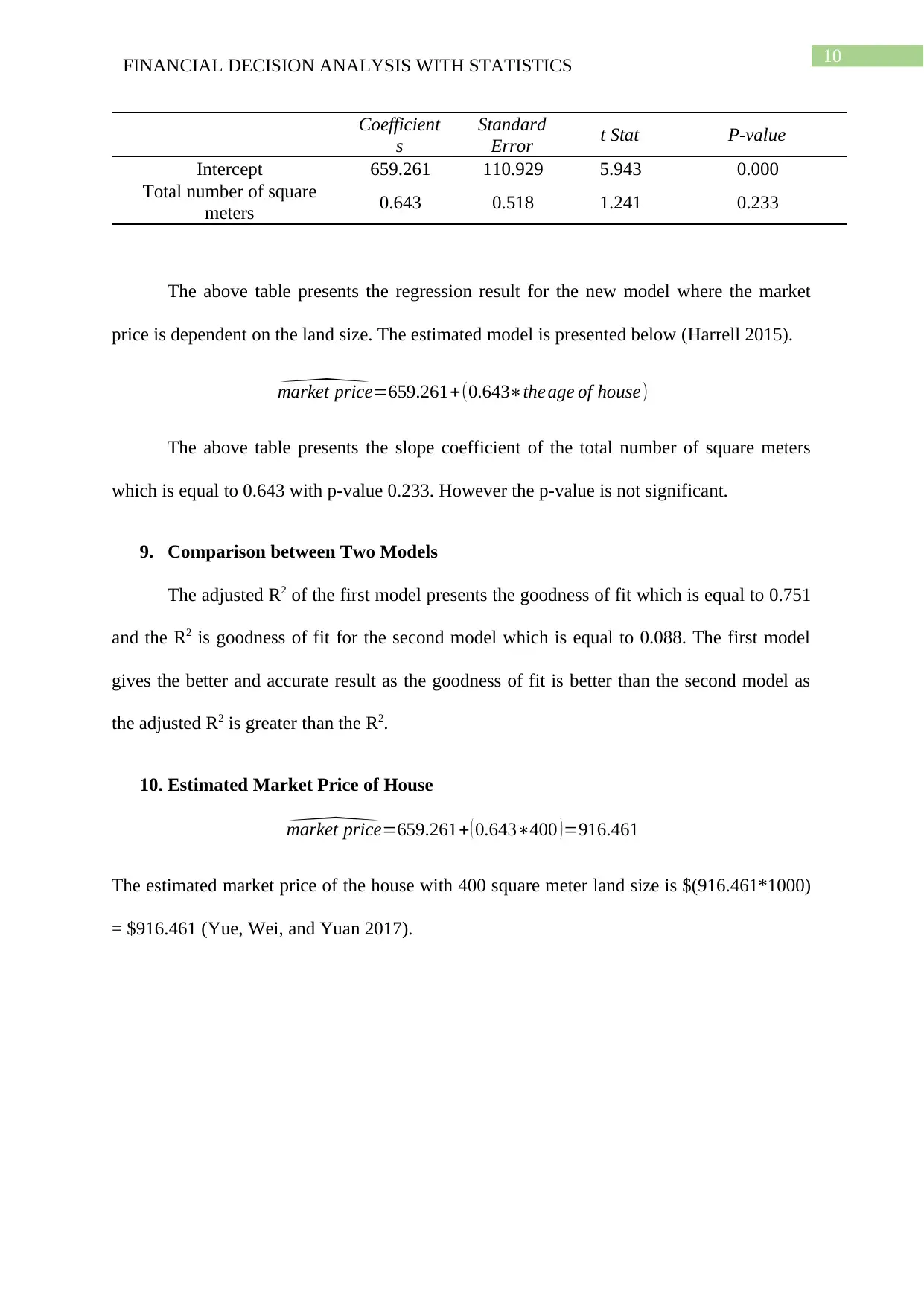
The above table presents the regression result for the new model where the market
price is dependent on the land size. The estimated model is presented below (Harrell 2015).
^market price=659.261+(0.643∗the age of house)
The above table presents the slope coefficient of the total number of square meters
which is equal to 0.643 with p-value 0.233. However the p-value is not significant.
9. Comparison between Two Models
The adjusted R2 of the first model presents the goodness of fit which is equal to 0.751
and the R2 is goodness of fit for the second model which is equal to 0.088. The first model
gives the better and accurate result as the goodness of fit is better than the second model as
the adjusted R2 is greater than the R2.
10. Estimated Market Price of House
^market price=659.261+ ( 0.643∗400 )=916.461
The estimated market price of the house with 400 square meter land size is $(916.461*1000)
= $916.461 (Yue, Wei, and Yuan 2017).
Coefficient
s
Standard
Error t Stat P-value
Intercept 659.261 110.929 5.943 0.000
Total number of square
meters 0.643 0.518 1.241 0.233
The above table presents the regression result for the new model where the market
price is dependent on the land size. The estimated model is presented below (Harrell 2015).
^market price=659.261+(0.643∗the age of house)
The above table presents the slope coefficient of the total number of square meters
which is equal to 0.643 with p-value 0.233. However the p-value is not significant.
9. Comparison between Two Models
The adjusted R2 of the first model presents the goodness of fit which is equal to 0.751
and the R2 is goodness of fit for the second model which is equal to 0.088. The first model
gives the better and accurate result as the goodness of fit is better than the second model as
the adjusted R2 is greater than the R2.
10. Estimated Market Price of House
^market price=659.261+ ( 0.643∗400 )=916.461
The estimated market price of the house with 400 square meter land size is $(916.461*1000)
= $916.461 (Yue, Wei, and Yuan 2017).
11FINANCIAL DECISION ANALYSIS WITH STATISTICS
Reference
Austin, P.C. and Steyerberg, E.W., 2015. The number of subjects per variable required in
linear regression analyses. Journal of clinical epidemiology, 68(6), pp.627-636.
Aydin, M. and Malcioglu, G., 2016. Financial development and economic growth
relationship: The case of OECD countries. Journal of Applied Research in Finance and
Economics, 2(1), pp.1-7.
Bivand, R. and Piras, G., 2015. Comparing implementations of estimation methods for spatial
econometrics. American Statistical Association.
Brooks, C., 2019. Introductory econometrics for finance. Cambridge university press.
Carroll, R.J., 2017. Transformation and weighting in regression. Routledge.
Chatterjee, S. and Hadi, A.S., 2015. Regression analysis by example. John Wiley & Sons.
Faraway, J.J., 2016. Linear models with R. Chapman and Hall/CRC.
Fumo, N. and Biswas, M.R., 2015. Regression analysis for prediction of residential energy
consumption. Renewable and sustainable energy reviews, 47, pp.332-343.
Gourieroux, C. and Jasiak, J., 2018. Financial econometrics: Problems, models, and methods.
Princeton University Press.
Harrell Jr, F.E., 2015. Regression modeling strategies: with applications to linear models,
logistic and ordinal regression, and survival analysis. Springer.
Lee, D.K., 2016. Alternatives to P value: confidence interval and effect size. Korean journal
of anesthesiology, 69(6), p.555.
Lewis-Beck, C. and Lewis-Beck, M., 2015. Applied regression: An introduction (Vol. 22).
Sage publications.
12FINANCIAL DECISION ANALYSIS WITH STATISTICS
McCullagh, P., 2018. Generalized linear models. Routledge.
Schober, P., Boer, C. and Schwarte, L.A., 2018. Correlation coefficients: appropriate use and
interpretation. Anesthesia & Analgesia, 126(5), pp.1763-1768.
Vogel, H.L., 2018. Financial Market Bubbles and Crashes: Features, Causes, and Effects.
Springer.
Yue, Y., Wei, M. and Yuan, S., 2017. Forecast related to linear regression of China’s tourism
market. Journal of Interdisciplinary Mathematics, 20(6-7), pp.1367-1371.
1 out of 13
Related Documents


Your All-in-One AI-Powered Toolkit for Academic Success.
+13062052269
info@desklib.com
Available 24*7 on WhatsApp / Email
![[object Object]](/_next/static/media/star-bottom.7253800d.svg)
Unlock your academic potential
© 2024 | Zucol Services PVT LTD | All rights reserved.