Data Analysis Report of Health and Population Statistics of East Asian and Pacific Countries
VerifiedAdded on 2023/06/11
|15
|2593
|166
AI Summary
This report analyses the vital statistics of East Asia and Pacific region from 2001 to 2015. The report includes one-variable and two-variable analysis, clustering and linear regression to improve the health of the region. The report concludes that there is high level of GNI per capita for the country having country code MAC and there are outliers in the distribution of Gross national income if analysed country wise.
Contribute Materials
Your contribution can guide someone’s learning journey. Share your
documents today.

Data Analysis Report of the Health and Population Statistics of East Asian And Pacific Countries
Name of the Student:
1 | P a g e
Name of the Student:
1 | P a g e
Secure Best Marks with AI Grader
Need help grading? Try our AI Grader for instant feedback on your assignments.
Table of Contents
1 Introduction.................................................................................................................................3
1.1 Authorisation and Purpose...............................................................................................3
1.2 Limitations.........................................................................................................................3
1.3 Scope.................................................................................................................................3
2 Data Setup..................................................................................................................................3
3 Exploratory Data Analysis.............................................................................................................4
3.1. One variable analysis............................................................................................................4
3.1.1 One Variable Analysis – 1...................................................................................................4
3.1.2 One Variable Analysis – 2...................................................................................................5
3.1.3 One Variable Analysis – 3...................................................................................................6
3.2 Two-variable analysis.............................................................................................................7
3.2.1 Two-variable analysis 1.......................................................................................................7
3.2.2 Two-variable analysis 2.......................................................................................................8
4 Advanced analysis........................................................................................................................9
4.1 Clustering...............................................................................................................................9
4.1.1 Brief explanation of k-means and clustering......................................................................9
4.1.2 Clustering Analysis..............................................................................................................9
4.2 Linear regression..................................................................................................................11
4.2.1 Brief definition of linear regression..................................................................................11
4.2.2 Linear Regression 1...........................................................................................................11
4.2.3 Linear Regression 2...........................................................................................................12
5 Conclusion................................................................................................................................14
6 Reflection...................................................................................................................................14
References...................................................................................................................................15
2 | P a g e
1 Introduction
1.1 Authorisation and Purpose
The study aims to analyse the vital statistics of East Asia and Pacific region from the year
2001 to the year 2015 by collecting the dataset from the World Bank. The implication of this
analysis will be done by government planners to improve the health of that region.
1.2 Limitations
The primary constraint of this study is that the research and analysis is limited for East Asia
and Pacific region only. Moreover, the data is collected from World Bank which is secondary of
nature and it is another limitation.
1.3 Scope
The present study consists of 26 attributes holding information about health of the above
mentioned region. Besides, the data contains information for a long time period of 15 years.
The analysis can be performed using statistical analysis and interpreting the graphs. However,
the data has lots of missing observations.
The analysis is proceeded through one-variable analyses, two-variable analyses. On the next
step, the data is clustered using k-means clustering technique and finally, the data is analysed
by fitting linear regression lines between two attributes.
1.4 Methodology
The information has been generated from World Bank. The dataset is quantitative in nature
and contains information about health for the time period of 2001 to 2015.
2 Data Setup
The data is loaded into the “R” program before the analysis. A pop-up window gets opened
after running the first line of the code and then the data file (in csv format) is selected by
inputting the location of the data file. The missing values are addressed in the first line of the
code as missing values.
At the second step, the necessary library files are loaded to the “R” program to perform the
required statistical analyses and to display all the graphical presentations.
3 | P a g e
Health0 <- read.csv(file.choose(), header = TRUE, sep = "," , na.strings = "..")
# Loading required library files
library(data.table)
library(reshape2)
library(psych)
library(ggplot2)
library(lattice)
library(dplyr)
3 Exploratory Data Analysis
3.1. One variable analysis
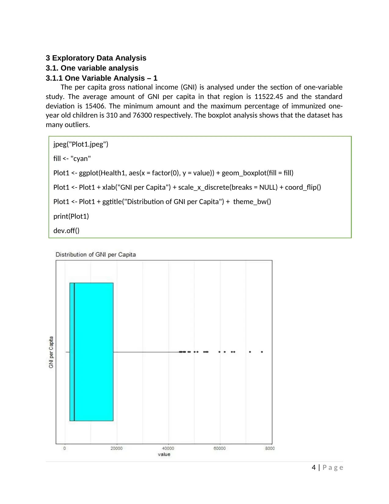
3.1.1 One Variable Analysis – 1
The per capita gross national income (GNI) is analysed under the section of one-variable
study. The average amount of GNI per capita in that region is 11522.45 and the standard
deviation is 15406. The minimum amount and the maximum percentage of immunized one-
year old children is 310 and 76300 respectively. The boxplot analysis shows that the dataset has
many outliers.
4 | P a g e
jpeg("Plot1.jpeg")
fill <- "cyan"
Plot1 <- ggplot(Health1, aes(x = factor(0), y = value)) + geom_boxplot(fill = fill)
Plot1 <- Plot1 + xlab("GNI per Capita") + scale_x_discrete(breaks = NULL) + coord_flip()
Plot1 <- Plot1 + ggtitle("Distribution of GNI per Capita") + theme_bw()
print(Plot1)
dev.off()
3.1. One variable analysis
3.1.1 One Variable Analysis – 1
The per capita gross national income (GNI) is analysed under the section of one-variable
study. The average amount of GNI per capita in that region is 11522.45 and the standard
deviation is 15406. The minimum amount and the maximum percentage of immunized one-
year old children is 310 and 76300 respectively. The boxplot analysis shows that the dataset has
many outliers.
4 | P a g e
jpeg("Plot1.jpeg")
fill <- "cyan"
Plot1 <- ggplot(Health1, aes(x = factor(0), y = value)) + geom_boxplot(fill = fill)
Plot1 <- Plot1 + xlab("GNI per Capita") + scale_x_discrete(breaks = NULL) + coord_flip()
Plot1 <- Plot1 + ggtitle("Distribution of GNI per Capita") + theme_bw()
print(Plot1)
dev.off()
Secure Best Marks with AI Grader
Need help grading? Try our AI Grader for instant feedback on your assignments.
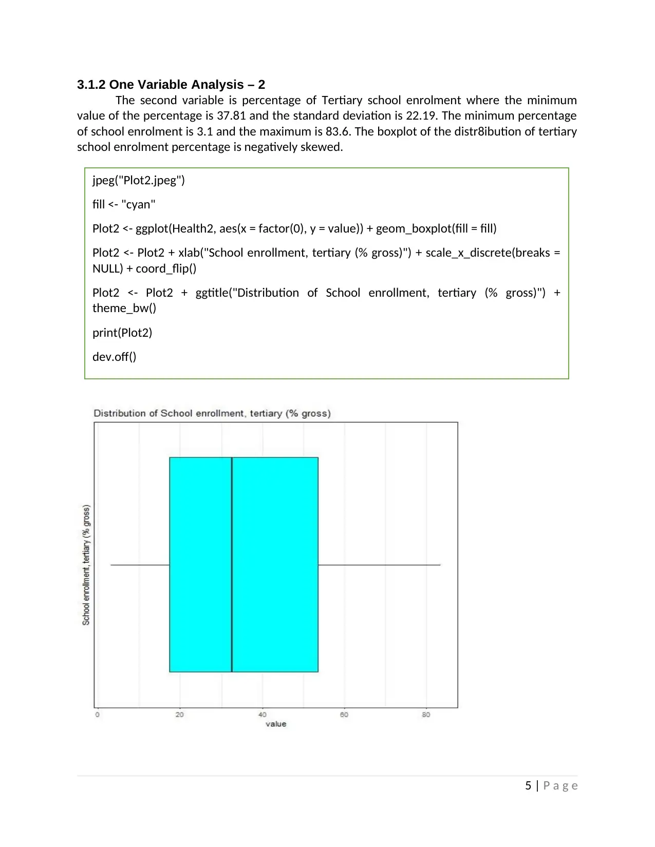
3.1.2 One Variable Analysis – 2
The second variable is percentage of Tertiary school enrolment where the minimum
value of the percentage is 37.81 and the standard deviation is 22.19. The minimum percentage
of school enrolment is 3.1 and the maximum is 83.6. The boxplot of the distr8ibution of tertiary
school enrolment percentage is negatively skewed.
5 | P a g e
jpeg("Plot2.jpeg")
fill <- "cyan"
Plot2 <- ggplot(Health2, aes(x = factor(0), y = value)) + geom_boxplot(fill = fill)
Plot2 <- Plot2 + xlab("School enrollment, tertiary (% gross)") + scale_x_discrete(breaks =
NULL) + coord_flip()
Plot2 <- Plot2 + ggtitle("Distribution of School enrollment, tertiary (% gross)") +
theme_bw()
print(Plot2)
dev.off()
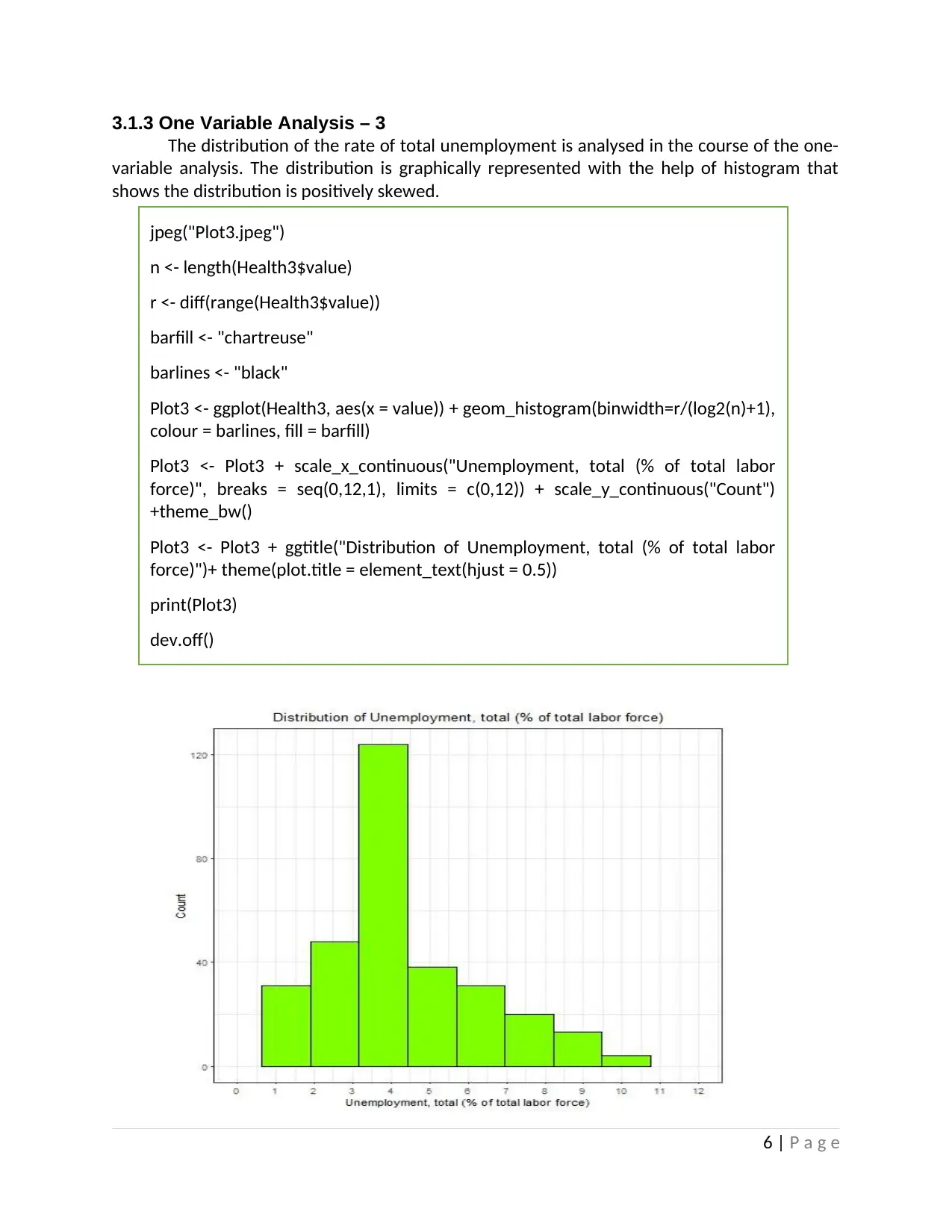
3.1.3 One Variable Analysis – 3
The distribution of the rate of total unemployment is analysed in the course of the one-
variable analysis. The distribution is graphically represented with the help of histogram that
shows the distribution is positively skewed.
6 | P a g e
jpeg("Plot3.jpeg")
n <- length(Health3$value)
r <- diff(range(Health3$value))
barfill <- "chartreuse"
barlines <- "black"
Plot3 <- ggplot(Health3, aes(x = value)) + geom_histogram(binwidth=r/(log2(n)+1),
colour = barlines, fill = barfill)
Plot3 <- Plot3 + scale_x_continuous("Unemployment, total (% of total labor
force)", breaks = seq(0,12,1), limits = c(0,12)) + scale_y_continuous("Count")
+theme_bw()
Plot3 <- Plot3 + ggtitle("Distribution of Unemployment, total (% of total labor
force)")+ theme(plot.title = element_text(hjust = 0.5))
print(Plot3)
dev.off()
3.2 Two-variable analysis
3.2.1 Two-variable analysis 1
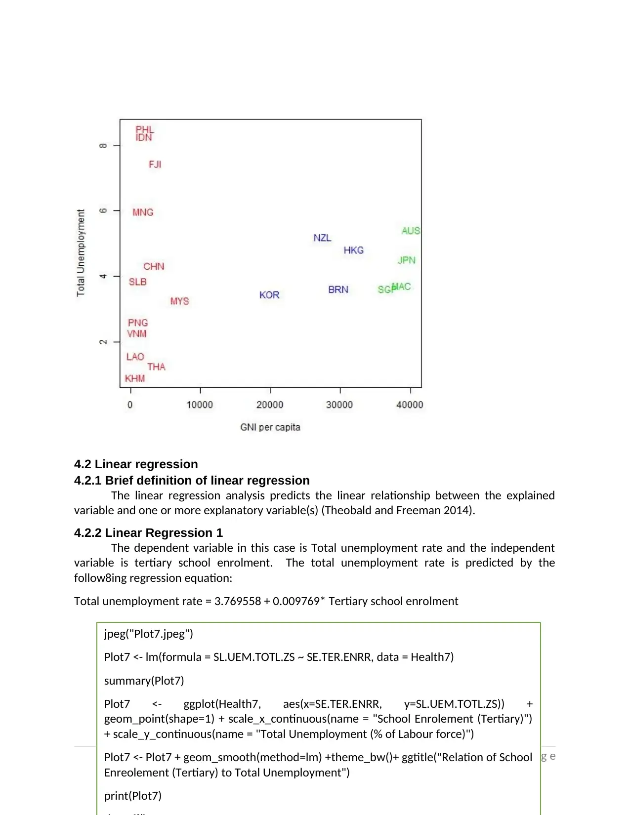
In the course of two-variable analysis, the Gross national income is analysed country wise
for the region and it is graphically represented by side-by-side Box-plot. The graph shows that
there has been huge variation in GNI during the time period of 2001 to 2015. The maximum
gross national income has been obtained for the country Macao SAR, China.
7 | P a g e
jpeg("Plot4.jpeg")
fill = "Orange"
Plot4 <- ggplot(Health4, aes(x = Health4$Country.Code, y =
Health4$value)) + geom_boxplot(fill = fill)
Plot4 <- Plot4 + scale_x_discrete(name = "Country") +
scale_y_continuous(name = "Gross National Income")+ theme_bw()
Plot4 <- Plot4 +theme(axis.text.x = element_text(angle = 90, hjust = 1)) +
ggtitle("Distribution of GNI per Capita")
print(Plot4)
dev.off()
3.2.1 Two-variable analysis 1
In the course of two-variable analysis, the Gross national income is analysed country wise
for the region and it is graphically represented by side-by-side Box-plot. The graph shows that
there has been huge variation in GNI during the time period of 2001 to 2015. The maximum
gross national income has been obtained for the country Macao SAR, China.
7 | P a g e
jpeg("Plot4.jpeg")
fill = "Orange"
Plot4 <- ggplot(Health4, aes(x = Health4$Country.Code, y =
Health4$value)) + geom_boxplot(fill = fill)
Plot4 <- Plot4 + scale_x_discrete(name = "Country") +
scale_y_continuous(name = "Gross National Income")+ theme_bw()
Plot4 <- Plot4 +theme(axis.text.x = element_text(angle = 90, hjust = 1)) +
ggtitle("Distribution of GNI per Capita")
print(Plot4)
dev.off()
Paraphrase This Document
Need a fresh take? Get an instant paraphrase of this document with our AI Paraphraser
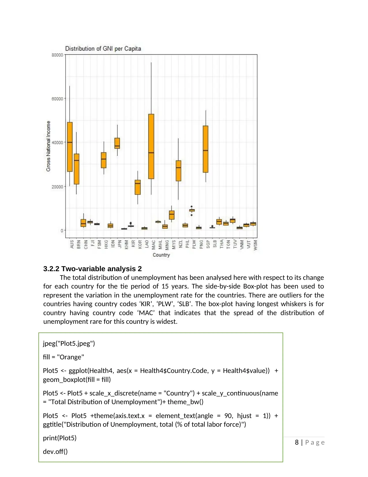
3.2.2 Two-variable analysis 2
The total distribution of unemployment has been analysed here with respect to its change
for each country for the tie period of 15 years. The side-by-side Box-plot has been used to
represent the variation in the unemployment rate for the countries. There are outliers for the
countries having country codes ‘KIR’, ‘PLW’, ‘SLB’. The box-plot having longest whiskers is for
country having country code ‘MAC’ that indicates that the spread of the distribution of
unemployment rare for this country is widest.
8 | P a g e
jpeg("Plot5.jpeg")
fill = "Orange"
Plot5 <- ggplot(Health4, aes(x = Health4$Country.Code, y = Health4$value)) +
geom_boxplot(fill = fill)
Plot5 <- Plot5 + scale_x_discrete(name = "Country") + scale_y_continuous(name
= "Total Distribution of Unemployment")+ theme_bw()
Plot5 <- Plot5 +theme(axis.text.x = element_text(angle = 90, hjust = 1)) +
ggtitle("Distribution of Unemployment, total (% of total labor force)")
print(Plot5)
dev.off()
4 Advanced
analysis
4.1 Clustering
4.1.1 Brief
explanation of k-
means and
clustering
Clustering
means segregating
the entire dataset
into smaller groups
having similar
characteristics. K-
means clustering is
a special type of
non-hierarchical
clustering
technique that uses
the centroid
distances for group
segmentation
(Oleiwi 2016). The
centroids are
initially selected and the data points are assigned into them on the basis of the nearest distance
from the centroid. The process is repeated until all the data points are assigned into groups
(Cohen et al. 2015).
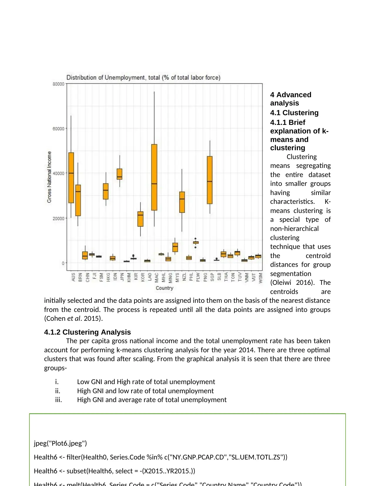
4.1.2 Clustering Analysis
The per capita gross national income and the total unemployment rate has been taken
account for performing k-means clustering analysis for the year 2014. There are three optimal
clusters that was found after scaling. From the graphical analysis it is seen that there are three
groups-
i. Low GNI and High rate of total unemployment
ii. High GNI and low rate of total unemployment
iii. High GNI and average rate of total unemployment
9 | P a g e
jpeg("Plot6.jpeg")
Health6 <- filter(Health0, Series.Code %in% c("NY.GNP.PCAP.CD","SL.UEM.TOTL.ZS"))
Health6 <- subset(Health6, select = -(X2015..YR2015.))
analysis
4.1 Clustering
4.1.1 Brief
explanation of k-
means and
clustering
Clustering
means segregating
the entire dataset
into smaller groups
having similar
characteristics. K-
means clustering is
a special type of
non-hierarchical
clustering
technique that uses
the centroid
distances for group
segmentation
(Oleiwi 2016). The
centroids are
initially selected and the data points are assigned into them on the basis of the nearest distance
from the centroid. The process is repeated until all the data points are assigned into groups
(Cohen et al. 2015).
4.1.2 Clustering Analysis
The per capita gross national income and the total unemployment rate has been taken
account for performing k-means clustering analysis for the year 2014. There are three optimal
clusters that was found after scaling. From the graphical analysis it is seen that there are three
groups-
i. Low GNI and High rate of total unemployment
ii. High GNI and low rate of total unemployment
iii. High GNI and average rate of total unemployment
9 | P a g e
jpeg("Plot6.jpeg")
Health6 <- filter(Health0, Series.Code %in% c("NY.GNP.PCAP.CD","SL.UEM.TOTL.ZS"))
Health6 <- subset(Health6, select = -(X2015..YR2015.))

10 | P a g e
Secure Best Marks with AI Grader
Need help grading? Try our AI Grader for instant feedback on your assignments.
4.2 Linear regression
4.2.1 Brief definition of linear regression
The linear regression analysis predicts the linear relationship between the explained
variable and one or more explanatory variable(s) (Theobald and Freeman 2014).
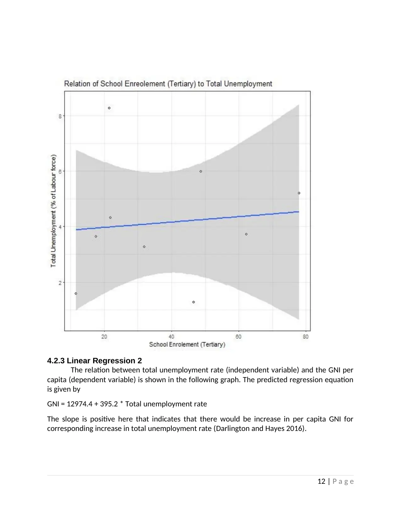
4.2.2 Linear Regression 1
The dependent variable in this case is Total unemployment rate and the independent
variable is tertiary school enrolment. The total unemployment rate is predicted by the
follow8ing regression equation:
Total unemployment rate = 3.769558 + 0.009769* Tertiary school enrolment
11 | P a g e
jpeg("Plot7.jpeg")
Plot7 <- lm(formula = SL.UEM.TOTL.ZS ~ SE.TER.ENRR, data = Health7)
summary(Plot7)
Plot7 <- ggplot(Health7, aes(x=SE.TER.ENRR, y=SL.UEM.TOTL.ZS)) +
geom_point(shape=1) + scale_x_continuous(name = "School Enrolement (Tertiary)")
+ scale_y_continuous(name = "Total Unemployment (% of Labour force)")
Plot7 <- Plot7 + geom_smooth(method=lm) +theme_bw()+ ggtitle("Relation of School
Enreolement (Tertiary) to Total Unemployment")
print(Plot7)
4.2.1 Brief definition of linear regression
The linear regression analysis predicts the linear relationship between the explained
variable and one or more explanatory variable(s) (Theobald and Freeman 2014).
4.2.2 Linear Regression 1
The dependent variable in this case is Total unemployment rate and the independent
variable is tertiary school enrolment. The total unemployment rate is predicted by the
follow8ing regression equation:
Total unemployment rate = 3.769558 + 0.009769* Tertiary school enrolment
11 | P a g e
jpeg("Plot7.jpeg")
Plot7 <- lm(formula = SL.UEM.TOTL.ZS ~ SE.TER.ENRR, data = Health7)
summary(Plot7)
Plot7 <- ggplot(Health7, aes(x=SE.TER.ENRR, y=SL.UEM.TOTL.ZS)) +
geom_point(shape=1) + scale_x_continuous(name = "School Enrolement (Tertiary)")
+ scale_y_continuous(name = "Total Unemployment (% of Labour force)")
Plot7 <- Plot7 + geom_smooth(method=lm) +theme_bw()+ ggtitle("Relation of School
Enreolement (Tertiary) to Total Unemployment")
print(Plot7)
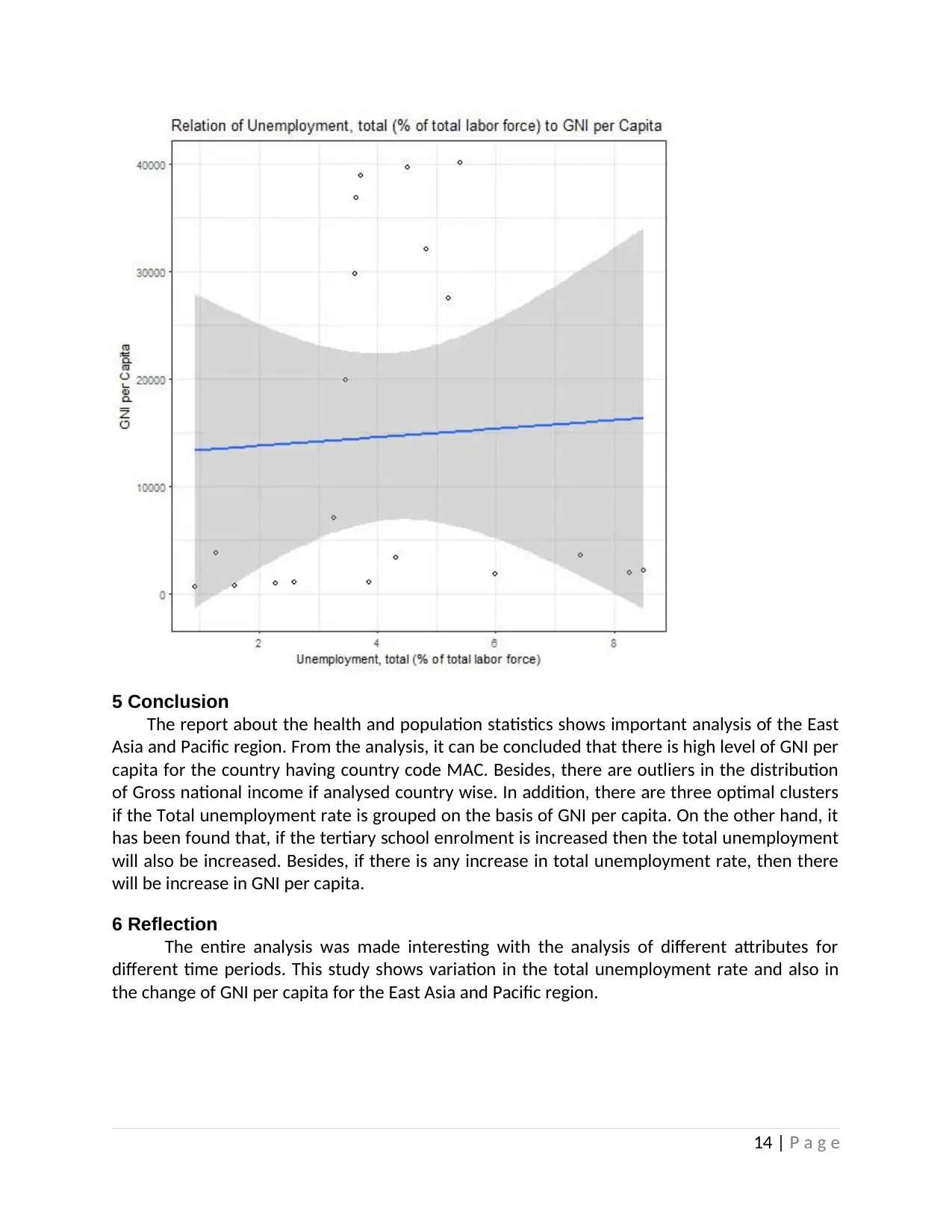
4.2.3 Linear Regression 2
The relation between total unemployment rate (independent variable) and the GNI per
capita (dependent variable) is shown in the following graph. The predicted regression equation
is given by
GNI = 12974.4 + 395.2 * Total unemployment rate
The slope is positive here that indicates that there would be increase in per capita GNI for
corresponding increase in total unemployment rate (Darlington and Hayes 2016).
12 | P a g e
13 | P a g e
jpeg("Plot8.jpeg")
Plot8 <- lm(formula = NY.GNP.PCAP.CD ~ SL.UEM.TOTL.ZS, data = Health7)
summary(Plot8)
Plot8 <- ggplot(Health7, aes(x=SL.UEM.TOTL.ZS, y=NY.GNP.PCAP.CD)) +
geom_point(shape=1) + scale_x_continuous(name = "Unemployment, total (%
of total labor force)") + scale_y_continuous(name = "GNI per Capita")
Plot8 <- Plot8 + geom_smooth(method=lm) +theme_bw()+ ggtitle("Relation of
Unemployment, total (% of total labor force) to GNI per Capita")
print(Plot8)
dev.off()
Paraphrase This Document
Need a fresh take? Get an instant paraphrase of this document with our AI Paraphraser
5 Conclusion
The report about the health and population statistics shows important analysis of the East
Asia and Pacific region. From the analysis, it can be concluded that there is high level of GNI per
capita for the country having country code MAC. Besides, there are outliers in the distribution
of Gross national income if analysed country wise. In addition, there are three optimal clusters
if the Total unemployment rate is grouped on the basis of GNI per capita. On the other hand, it
has been found that, if the tertiary school enrolment is increased then the total unemployment
will also be increased. Besides, if there is any increase in total unemployment rate, then there
will be increase in GNI per capita.
6 Reflection
The entire analysis was made interesting with the analysis of different attributes for
different time periods. This study shows variation in the total unemployment rate and also in
the change of GNI per capita for the East Asia and Pacific region.
14 | P a g e
References
Cohen, M.B., Elder, S., Musco, C., Musco, C. and Persu, M., 2015, June. Dimensionality
reduction for k-means clustering and low rank approximation. In Proceedings of the forty-
seventh annual ACM symposium on Theory of computing (pp. 163-172). ACM.
Darlington, R.B. and Hayes, A.F., 2016. Regression analysis and linear models: Concepts,
applications, and implementation. Guilford Publications.
Oleiwi, W.K., 2016. Using the Fuzzy Logic to Find Optimal Centers of Clusters of K-means.
International Journal of Electrical and Computer Engineering, 6(6), p.3068.
Theobald, R. and Freeman, S., 2014. Is it the intervention or the students? Using linear
regression to control for student characteristics in undergraduate STEM education research.
CBE-Life Sciences Education, 13(1), pp.41-48.
15 | P a g e
1 out of 15
Related Documents


Your All-in-One AI-Powered Toolkit for Academic Success.
+13062052269
info@desklib.com
Available 24*7 on WhatsApp / Email
![[object Object]](/_next/static/media/star-bottom.7253800d.svg)
Unlock your academic potential
© 2024 | Zucol Services PVT LTD | All rights reserved.