Regression Analysis and Salary Prediction

This assignment delves into the analysis of student salaries using regression models. It examines the influence of variables like ATAR scores, satisfaction levels, and university location on salary outcomes. Students are tasked with interpreting regression coefficients, assessing model significance, and utilizing the model to predict salaries based on given ATAR and satisfaction values. Additionally, they need to evaluate the linearity and normality of the data.

Quantitative methods 1
Name:
Institution:
Date:
Quantitative methods

Quantitative methods 2
QUESTION A
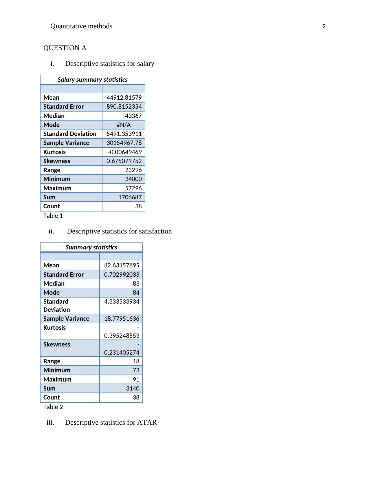
i. Descriptive statistics for salary
Salary summary statistics
Mean 44912.81579
Standard Error 890.8152354
Median 43367
Mode #N/A
Standard Deviation 5491.353911
Sample Variance 30154967.78
Kurtosis -0.00649469
Skewness 0.675079752
Range 23296
Minimum 34000
Maximum 57296
Sum 1706687
Count 38
Table 1
ii. Descriptive statistics for satisfaction
Summary statistics
Mean 82.63157895
Standard Error 0.702992033
Median 83
Mode 84
Standard
Deviation
4.333533934
Sample Variance 18.77951636
Kurtosis -
0.395248553
Skewness -
0.231405274
Range 18
Minimum 73
Maximum 91
Sum 3140
Count 38
Table 2
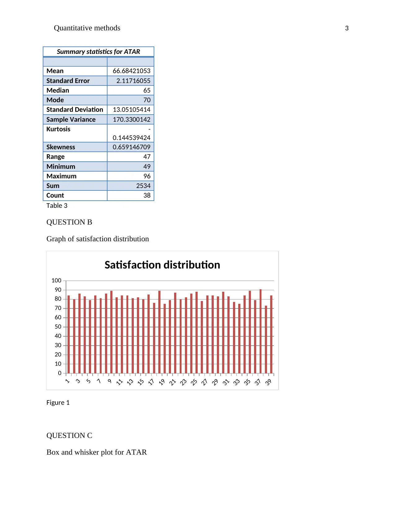
iii. Descriptive statistics for ATAR

Quantitative methods 3
Summary statistics for ATAR
Mean 66.68421053
Standard Error 2.11716055
Median 65
Mode 70
Standard Deviation 13.05105414
Sample Variance 170.3300142
Kurtosis -
0.144539424
Skewness 0.659146709
Range 47
Minimum 49
Maximum 96
Sum 2534
Count 38
Table 3
QUESTION B
Graph of satisfaction distribution
1
3
5
7
9
11
13
15
17
19
21
23
25
27
29
31
33
35
37
39
0
10
20
30
40
50
60
70
80
90
100
Satisfaction distribution
Figure 1
QUESTION C
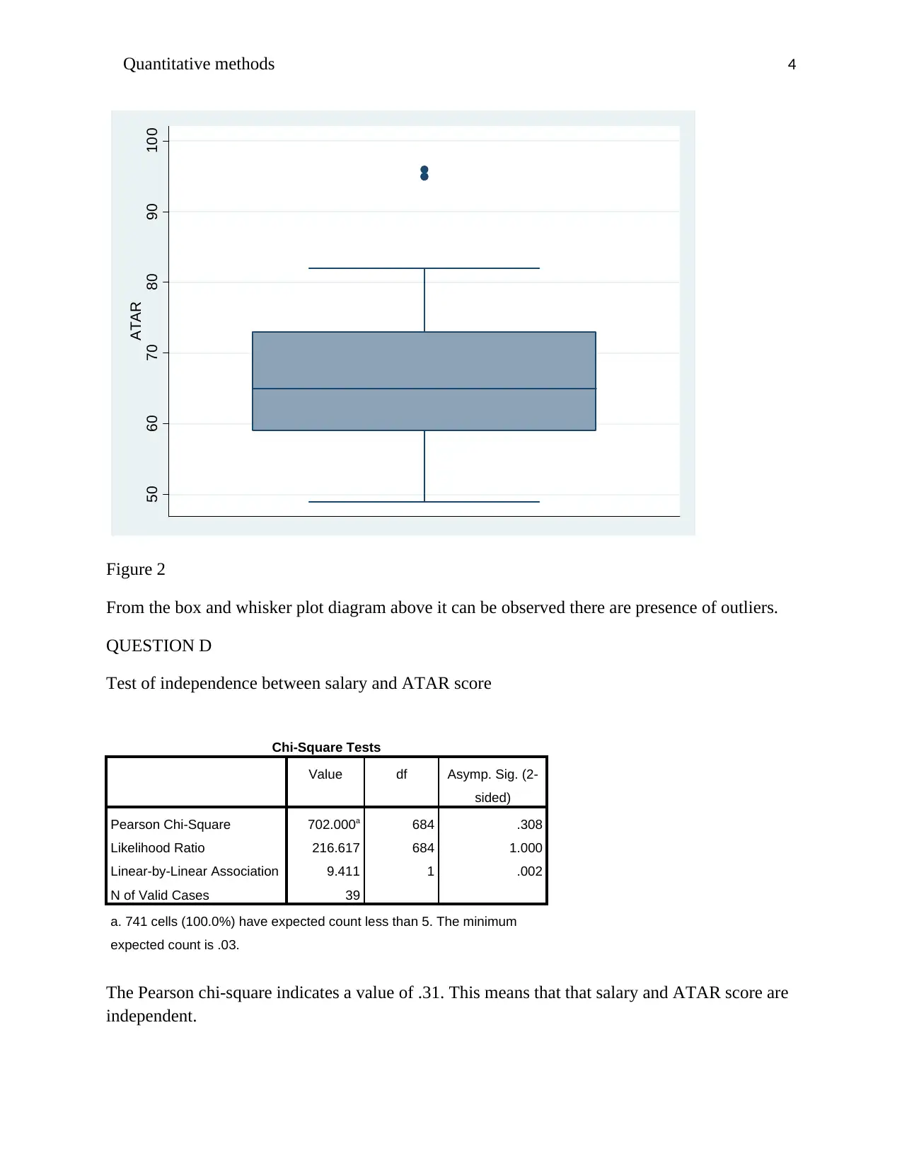
Box and whisker plot for ATAR

Quantitative methods 4
50 60 70 80 90 100
ATAR
Figure 2
From the box and whisker plot diagram above it can be observed there are presence of outliers.
QUESTION D
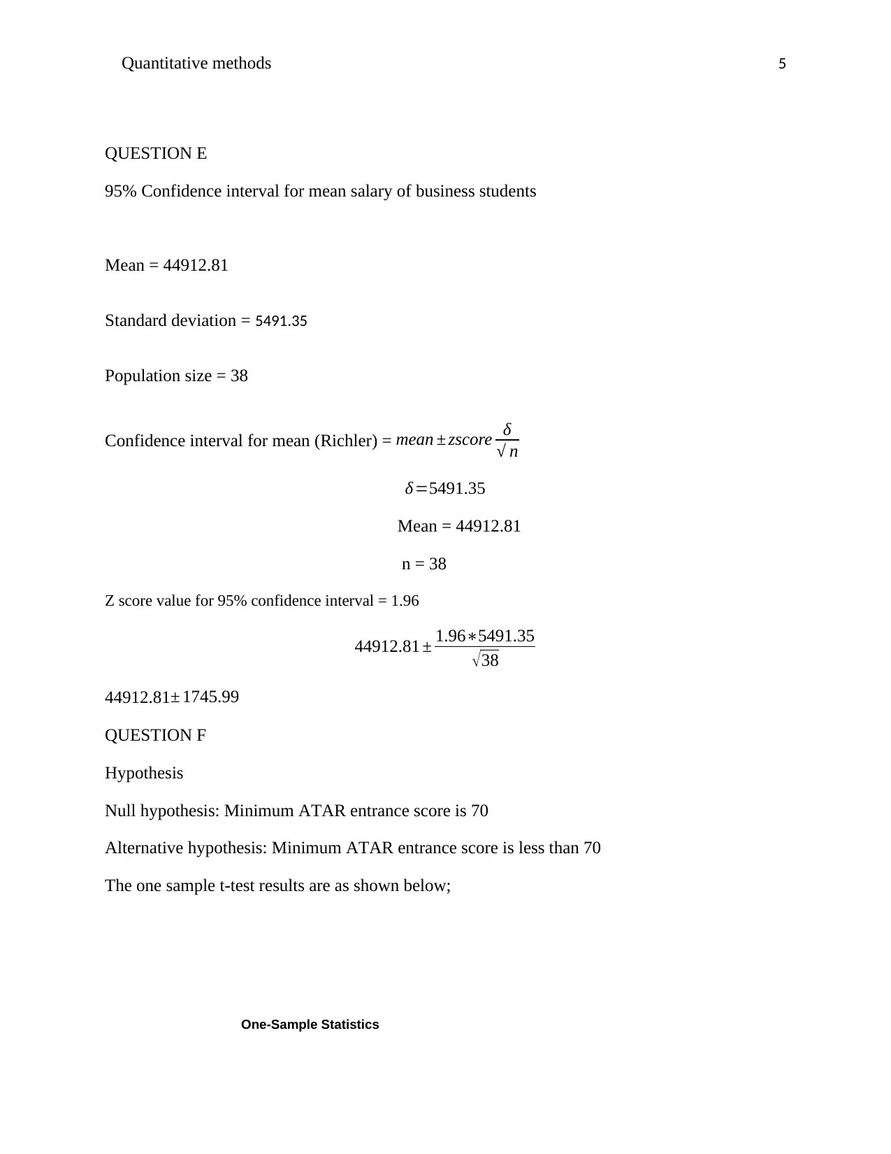
Test of independence between salary and ATAR score
Chi-Square Tests
Value df Asymp. Sig. (2-
sided)
Pearson Chi-Square 702.000a 684 .308
Likelihood Ratio 216.617 684 1.000
Linear-by-Linear Association 9.411 1 .002
N of Valid Cases 39
a. 741 cells (100.0%) have expected count less than 5. The minimum
expected count is .03.
The Pearson chi-square indicates a value of .31. This means that that salary and ATAR score are
independent.

Quantitative methods 5
QUESTION E
95% Confidence interval for mean salary of business students
Mean = 44912.81
Standard deviation = 5491.35
Population size = 38
Confidence interval for mean (Richler) = mean ± zscore δ
√ n
δ=5491.35
Mean = 44912.81
n = 38
Z score value for 95% confidence interval = 1.96
44912.81 ± 1.96∗5491.35
√38
44912.81± 1745.99
QUESTION F
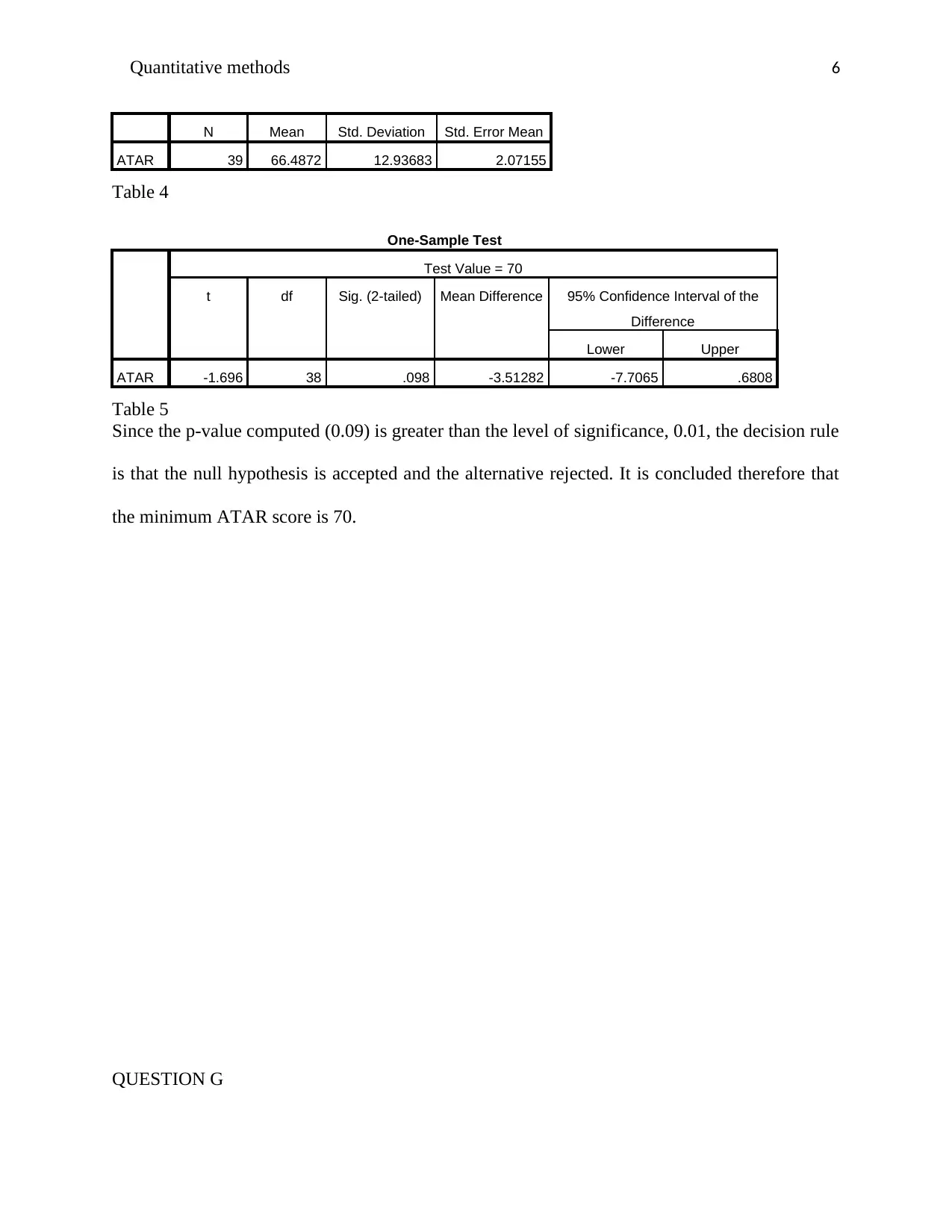
Hypothesis
Null hypothesis: Minimum ATAR entrance score is 70
Alternative hypothesis: Minimum ATAR entrance score is less than 70
The one sample t-test results are as shown below;
One-Sample Statistics

Quantitative methods 6
N Mean Std. Deviation Std. Error Mean
ATAR 39 66.4872 12.93683 2.07155
Table 4
One-Sample Test
Test Value = 70
t df Sig. (2-tailed) Mean Difference 95% Confidence Interval of the
Difference
Lower Upper
ATAR -1.696 38 .098 -3.51282 -7.7065 .6808
Table 5
Since the p-value computed (0.09) is greater than the level of significance, 0.01, the decision rule
is that the null hypothesis is accepted and the alternative rejected. It is concluded therefore that
the minimum ATAR score is 70.
QUESTION G

Quantitative methods 7
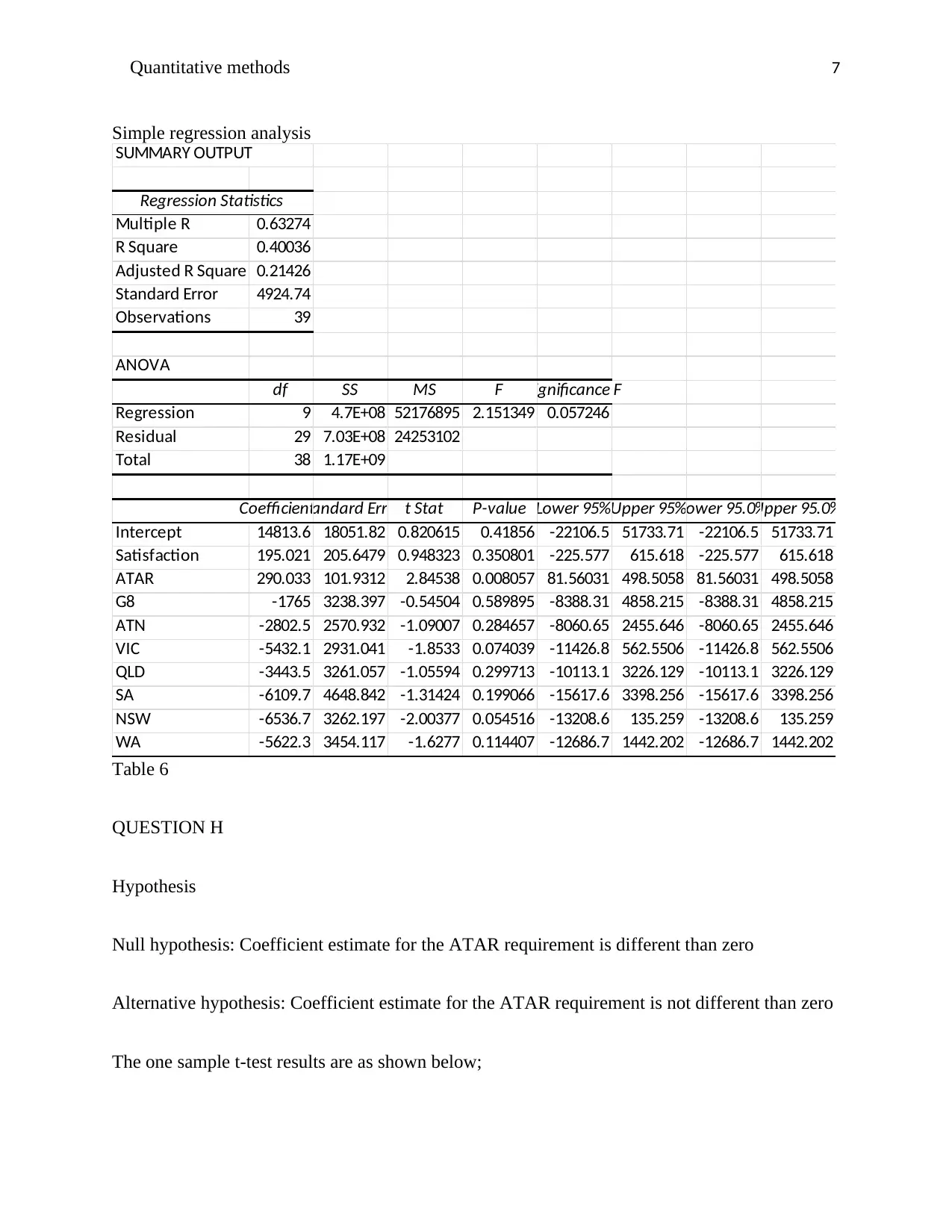
Simple regression analysis
SUMMARY OUTPUT
Regression Statistics
Multiple R 0.63274
R Square 0.40036
Adjusted R Square 0.21426
Standard Error 4924.74
Observations 39
ANOVA
df SS MS F Significance F
Regression 9 4.7E+08 52176895 2.151349 0.057246
Residual 29 7.03E+08 24253102
Total 38 1.17E+09
CoefficientsStandard Error t Stat P-value Lower 95%Upper 95%Lower 95.0%Upper 95.0%
Intercept 14813.6 18051.82 0.820615 0.41856 -22106.5 51733.71 -22106.5 51733.71
Satisfaction 195.021 205.6479 0.948323 0.350801 -225.577 615.618 -225.577 615.618
ATAR 290.033 101.9312 2.84538 0.008057 81.56031 498.5058 81.56031 498.5058
G8 -1765 3238.397 -0.54504 0.589895 -8388.31 4858.215 -8388.31 4858.215
ATN -2802.5 2570.932 -1.09007 0.284657 -8060.65 2455.646 -8060.65 2455.646
VIC -5432.1 2931.041 -1.8533 0.074039 -11426.8 562.5506 -11426.8 562.5506
QLD -3443.5 3261.057 -1.05594 0.299713 -10113.1 3226.129 -10113.1 3226.129
SA -6109.7 4648.842 -1.31424 0.199066 -15617.6 3398.256 -15617.6 3398.256
NSW -6536.7 3262.197 -2.00377 0.054516 -13208.6 135.259 -13208.6 135.259
WA -5622.3 3454.117 -1.6277 0.114407 -12686.7 1442.202 -12686.7 1442.202
Table 6
QUESTION H
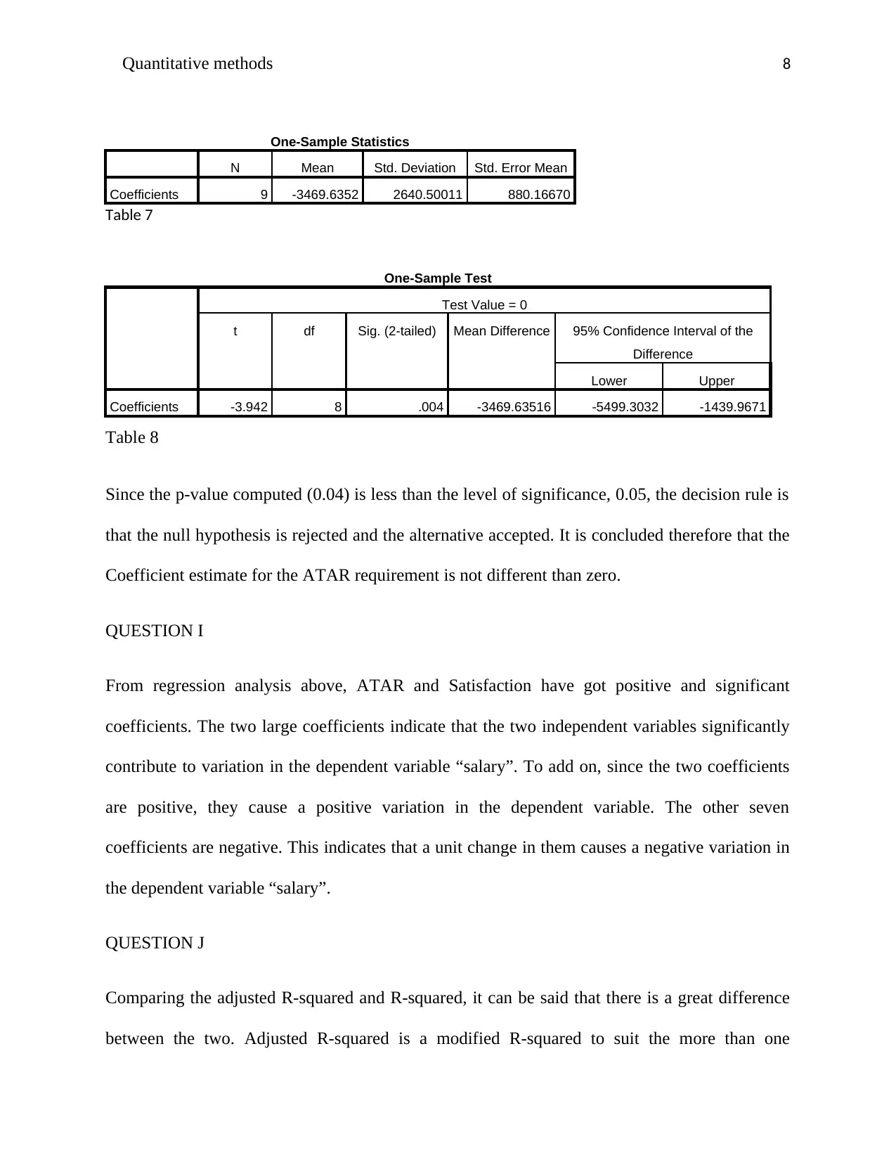
Hypothesis
Null hypothesis: Coefficient estimate for the ATAR requirement is different than zero
Alternative hypothesis: Coefficient estimate for the ATAR requirement is not different than zero
The one sample t-test results are as shown below;

Quantitative methods 8
One-Sample Statistics
N Mean Std. Deviation Std. Error Mean
Coefficients 9 -3469.6352 2640.50011 880.16670
Table 7
One-Sample Test
Test Value = 0
t df Sig. (2-tailed) Mean Difference 95% Confidence Interval of the
Difference
Lower Upper
Coefficients -3.942 8 .004 -3469.63516 -5499.3032 -1439.9671
Table 8
Since the p-value computed (0.04) is less than the level of significance, 0.05, the decision rule is
that the null hypothesis is rejected and the alternative accepted. It is concluded therefore that the
Coefficient estimate for the ATAR requirement is not different than zero.
QUESTION I
From regression analysis above, ATAR and Satisfaction have got positive and significant
coefficients. The two large coefficients indicate that the two independent variables significantly
contribute to variation in the dependent variable “salary”. To add on, since the two coefficients
are positive, they cause a positive variation in the dependent variable. The other seven
coefficients are negative. This indicates that a unit change in them causes a negative variation in
the dependent variable “salary”.
QUESTION J
Comparing the adjusted R-squared and R-squared, it can be said that there is a great difference
between the two. Adjusted R-squared is a modified R-squared to suit the more than one

Quantitative methods 9
independent variable. It is less than R-squared because the parameters that have been fitted in the
model are more than one.
QUESTION K
Is the model statistically significant?
From the p-value computed (0.06), it can be concluded that the model is statistically significant.
This is because this value is greater than the level of significance which is 0.05.
QUESTION L
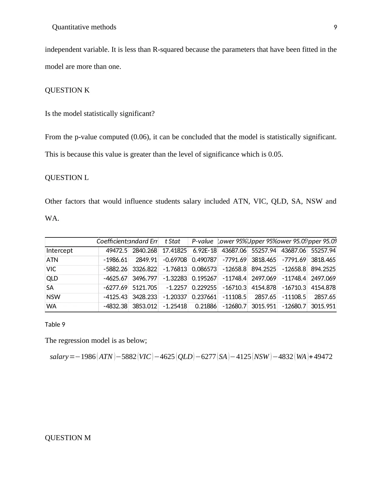
Other factors that would influence students salary included ATN, VIC, QLD, SA, NSW and
WA.
CoefficientsStandard Error t Stat P-value Lower 95%Upper 95%Lower 95.0%Upper 95.0%
Intercept 49472.5 2840.268 17.41825 6.92E-18 43687.06 55257.94 43687.06 55257.94
ATN -1986.61 2849.91 -0.69708 0.490787 -7791.69 3818.465 -7791.69 3818.465
VIC -5882.26 3326.822 -1.76813 0.086573 -12658.8 894.2525 -12658.8 894.2525
QLD -4625.67 3496.797 -1.32283 0.195267 -11748.4 2497.069 -11748.4 2497.069
SA -6277.69 5121.705 -1.2257 0.229255 -16710.3 4154.878 -16710.3 4154.878
NSW -4125.43 3428.233 -1.20337 0.237661 -11108.5 2857.65 -11108.5 2857.65
WA -4832.38 3853.012 -1.25418 0.21886 -12680.7 3015.951 -12680.7 3015.951
Table 9
The regression model is as below;
salary=−1986 ( ATN ) −5882 ( VIC ) −4625 ( QLD ) −6277 ( SA ) −4125 ( NSW ) −4832 ( WA ) + 49472
QUESTION M

Quantitative methods 10
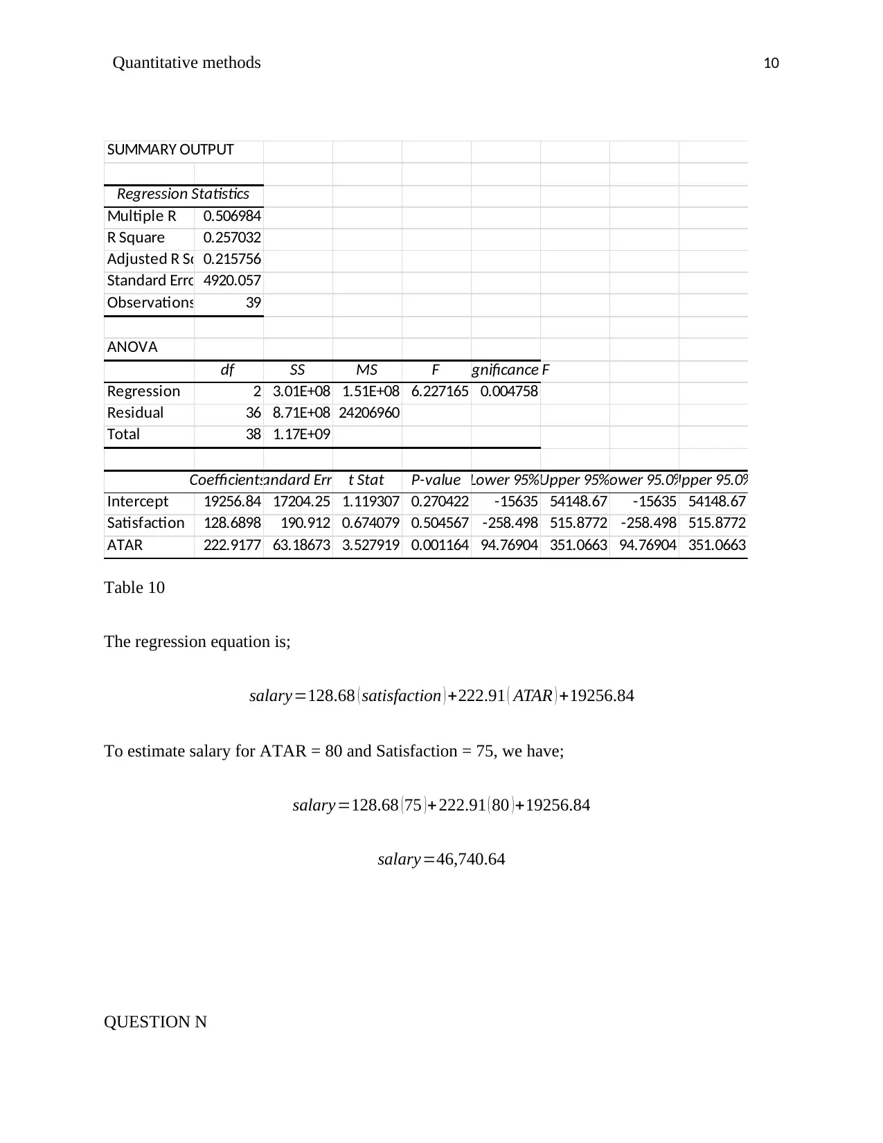
SUMMARY OUTPUT
Regression Statistics
Multiple R 0.506984
R Square 0.257032
Adjusted R Square0.215756
Standard Error4920.057
Observations 39
ANOVA
df SS MS F Significance F
Regression 2 3.01E+08 1.51E+08 6.227165 0.004758
Residual 36 8.71E+08 24206960
Total 38 1.17E+09
CoefficientsStandard Error t Stat P-value Lower 95%Upper 95%Lower 95.0%Upper 95.0%
Intercept 19256.84 17204.25 1.119307 0.270422 -15635 54148.67 -15635 54148.67
Satisfaction 128.6898 190.912 0.674079 0.504567 -258.498 515.8772 -258.498 515.8772
ATAR 222.9177 63.18673 3.527919 0.001164 94.76904 351.0663 94.76904 351.0663
Table 10
The regression equation is;
salary=128.68 ( satisfaction ) +222.91 ( ATAR ) +19256.84
To estimate salary for ATAR = 80 and Satisfaction = 75, we have;
salary=128.68 ( 75 ) +222.91 ( 80 ) +19256.84
salary=46,740.64
QUESTION N

Quantitative methods 11
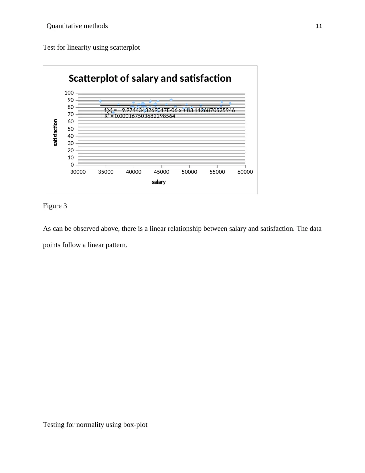
Test for linearity using scatterplot
30000 35000 40000 45000 50000 55000 60000
0
10
20
30
40
50
60
70
80
90
100
f(x) = − 9.9744343269017E-06 x + 83.1126870525946
R² = 0.000167503682298564
Scatterplot of salary and satisfaction
salary
satisfaction
Figure 3
As can be observed above, there is a linear relationship between salary and satisfaction. The data
points follow a linear pattern.
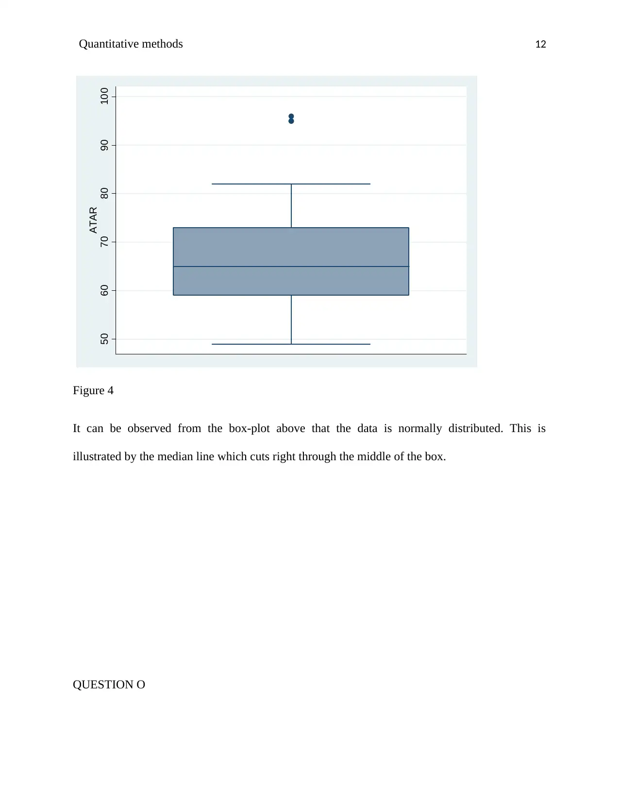
Testing for normality using box-plot

Quantitative methods 12
50 60 70 80 90 100
ATAR
Figure 4
It can be observed from the box-plot above that the data is normally distributed. This is
illustrated by the median line which cuts right through the middle of the box.
QUESTION O

Quantitative methods 13
35,000 40,000 45,000 50,000 55,000 60,000
Salary
Figure 5
As can be observed from figure 5 above, salaries among the students is not normally distributed.
To achieve normality, the data across the universities should be collected through simple random
sampling.