Regression Analysis | Assignment-1

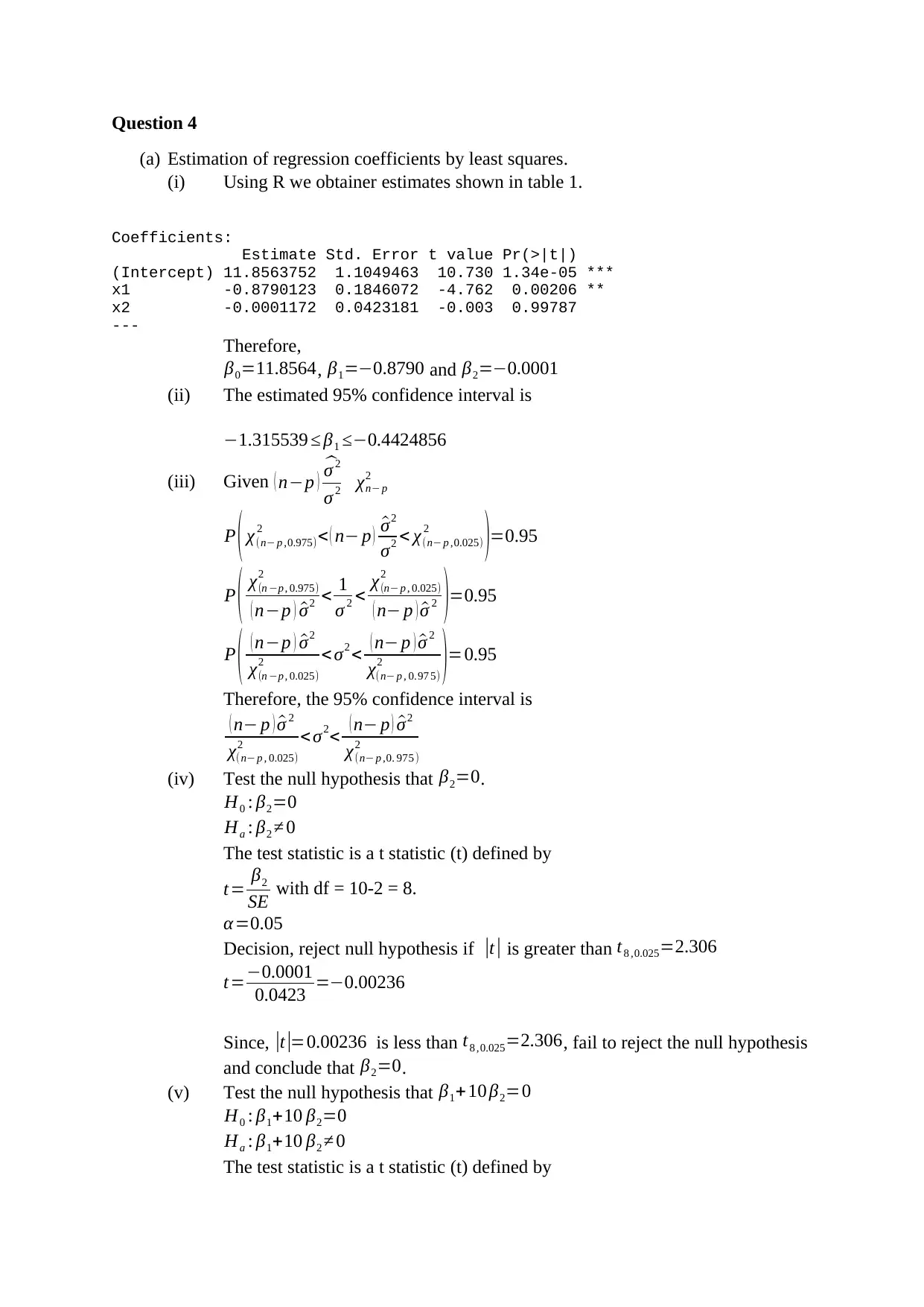
Question 4
(a) Estimation of regression coefficients by least squares.
(i) Using R we obtainer estimates shown in table 1.
Coefficients:
Estimate Std. Error t value Pr(>|t|)
(Intercept) 11.8563752 1.1049463 10.730 1.34e-05 ***
x1 -0.8790123 0.1846072 -4.762 0.00206 **
x2 -0.0001172 0.0423181 -0.003 0.99787
---
Therefore,
β0=11.8564, β1=−0.8790 and β2=−0.0001
(ii) The estimated 95% confidence interval is
−1.315539 ≤ β1 ≤−0.4424856
(iii) Given ( n−p ) ^σ 2
σ 2 χn− p
2
P ( χ(n− p ,0.975)
2 < ( n− p ) ^σ2
σ2 < χ(n− p ,0.025)
2
)=0.95
P ( χ(n −p , 0.975)
2
( n−p ) ^σ2 < 1
σ 2 < χ(n− p , 0.025)
2
( n− p ) ^σ 2 )=0.95
P ( ( n−p ) ^σ2
χ(n −p , 0.025)
2 < σ2 < ( n− p ) ^σ 2
χ(n− p , 0.97 5)
2 )=0.95
Therefore, the 95% confidence interval is
( n− p ) ^σ 2
χ(n− p , 0.025)
2 < σ2< ( n− p ) ^σ2
χ(n− p ,0. 975 )
2
(iv) Test the null hypothesis that β2=0.
H0 : β2=0
Ha : β2 ≠ 0
The test statistic is a t statistic (t) defined by
t= β2
SE with df = 10-2 = 8.
α=0.05
Decision, reject null hypothesis if |t | is greater than t8 ,0.025=2.306
t=−0.0001
0.0423 =−0.00236
Since, |t |=0.00236 is less than t8 ,0.025=2.306, fail to reject the null hypothesis
and conclude that β2=0.
(v) Test the null hypothesis that β1+10 β2=0
H0 : β1+10 β2=0
Ha : β1+10 β2 ≠ 0
The test statistic is a t statistic (t) defined by

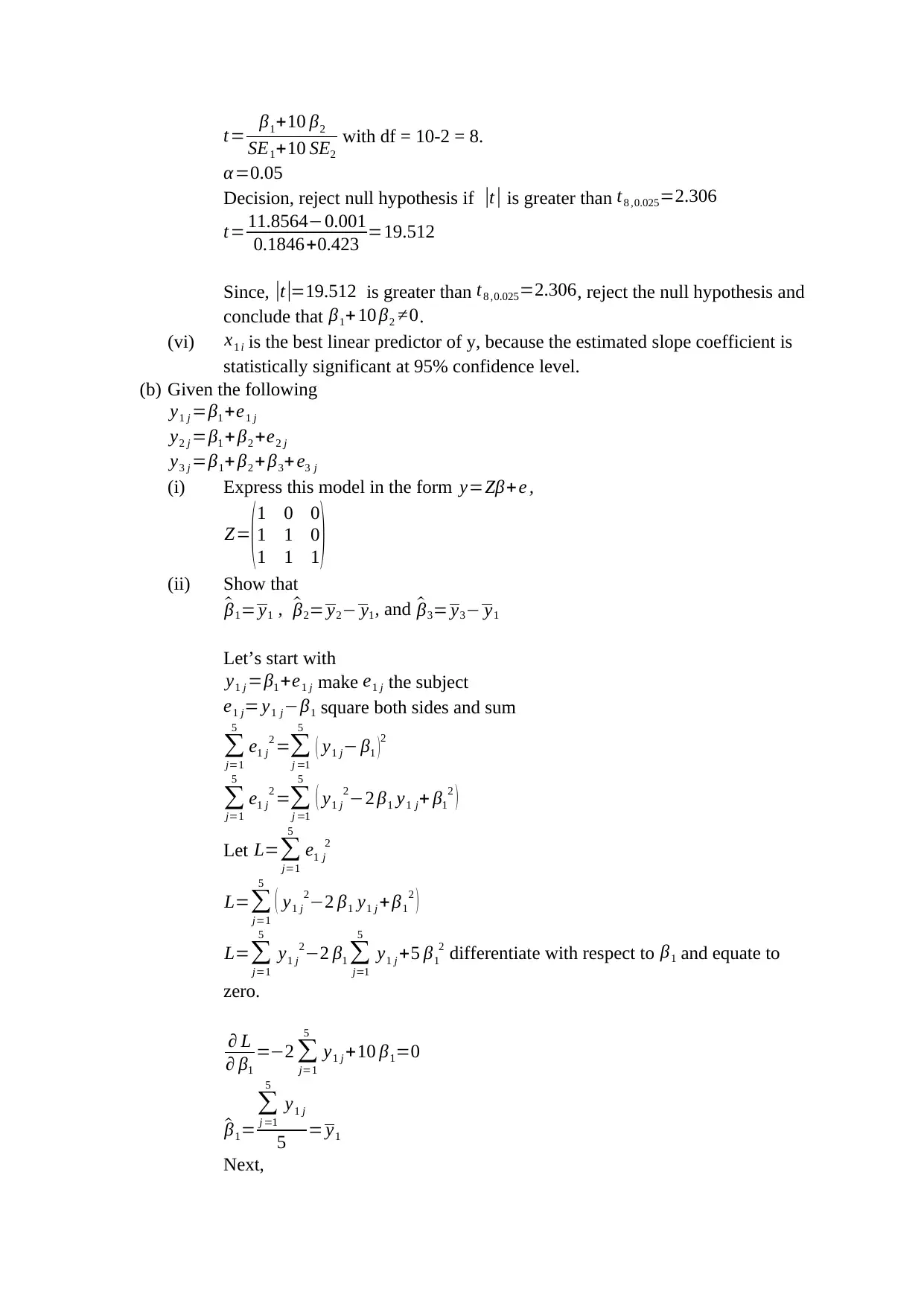
t= β1+10 β2
SE1+10 SE2
with df = 10-2 = 8.
α=0.05
Decision, reject null hypothesis if |t | is greater than t8 ,0.025=2.306
t= 11.8564−0.001
0.1846+0.423 =19.512
Since, |t |=19.512 is greater than t8 ,0.025=2.306, reject the null hypothesis and
conclude that β1+ 10 β2 ≠0.
(vi) x1 i is the best linear predictor of y, because the estimated slope coefficient is
statistically significant at 95% confidence level.
(b) Given the following
y1 j =β1 +e1 j
y2 j =β1 + β2 +e2 j
y3 j =β1+ β2 + β3+ e3 j
(i) Express this model in the form y=Zβ+e ,
Z=
(1 0 0
1 1 0
1 1 1)
(ii) Show that
^β1= y1 , ^β2= y2− y1, and ^β3= y3− y1
Let’s start with
y1 j =β1 +e1 j make e1 j the subject
e1 j= y1 j−β1 square both sides and sum
∑
j=1
5
e1 j
2 =∑
j =1
5
( y1 j− β1 )2
∑
j=1
5
e1 j
2 =∑
j =1
5
( y1 j
2−2 β1 y1 j+ β1
2 )
Let L=∑
j=1
5
e1 j
2
L=∑
j=1
5
( y1 j
2−2 β1 y1 j + β1
2 )
L=∑
j=1
5
y1 j
2−2 β1 ∑
j=1
5
y1 j +5 β1
2 differentiate with respect to β1 and equate to
zero.
∂ L
∂ β1
=−2 ∑
j=1
5
y1 j +10 β1=0
^β1=
∑
j =1
5
y1 j
5 = y1
Next,

y2 j =β1 + β2 +e2 j make e1 j the subject
e2 j= y2 j− y1−β2 square both sides and sum
∑
j=1
5
e2 j
2 =∑
j =1
5
( y2 j− y1−β2 )2
∑
j=1
5
e2 j
2 =∑
j =1
5
( y2 j
2−2 ( y1−β2 ) y2 j+ ( y1−β2 )2
)
Let L=∑
j=1
5
e2 j
2
L=∑
j=1
5
( y2 j
2−2 ( y1− β2 ) y2 j + ( y1− β2 ) 2
)
L=∑
j=1
5
y2 j
2−2 ( y1−β2 )∑
j=1
5
y2 j +5 ( y1
2−2 β2 y1 + β2
2 ) differentiate with respect to
β2 and equate to zero.
∂ L
∂ β1
=2∑
j=1
5
y2 j−10 y1 +10 β2=0
^β2=
∑
j =1
5
y2 j
5 − y1= y2− y1
Finally,
y3 j =β1+ β2 + β3+ e3 j make e1 j the subject
e3 j= y3 j− y2− β3 square both sides and sum
∑
j=1
5
e3 j
2=∑
j=1
5
( y3 j − y2−β3 )2
∑
j=1
5
e3 j
2=∑
j=1
5
( y3 j
2−2 ( y2−β3 ) y3 j + ( y2−β3 )2
)
Let L=∑
j=1
5
e3 j
2
L=∑
j=1
5
( y3 j
2−2 ( y2 −β3 ) y3 j + ( y2−β3 )2
)
L=∑
j=1
5
y3 j
2−2 ( y2−β3 ) ∑
j =1
5
y3 j +5 ( y2
2−2 β3 y2 +β3
2 ) differentiate with respect to
β3 and equate to zero.
∂ L
∂ β1
=2∑
j=1
5
y3 j−10 y2 +10 β3=0
^β2=
∑
j =1
5
y3 j
5 − y2= y3 − y2
(iii) Using R we obtain the column means for the data and thus we have the
estimates as follows:

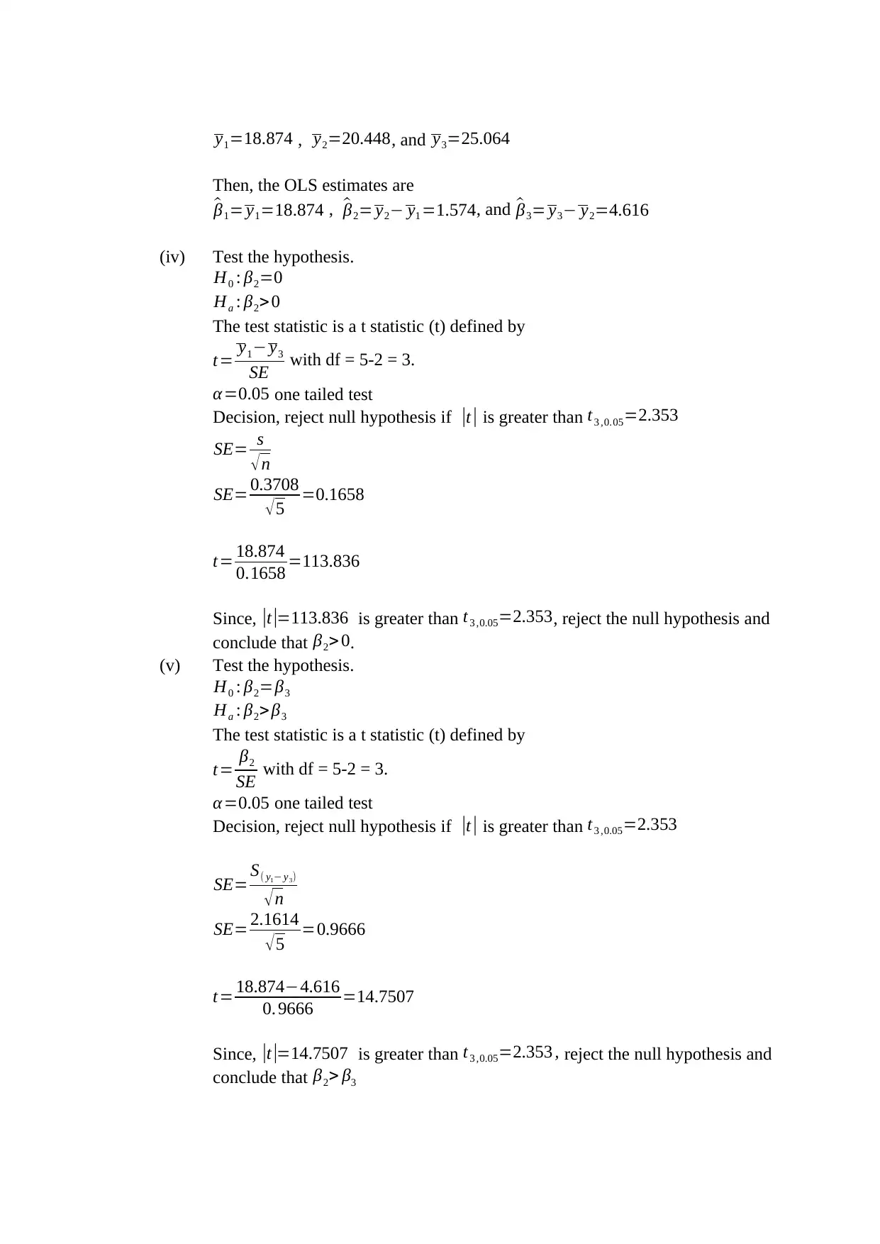
y1=18.874 , y2=20.448, and y3=25.064
Then, the OLS estimates are
^β1= y1=18.874 , ^β2= y2− y1 =1.574, and ^β3= y3− y2=4.616
(iv) Test the hypothesis.
H0 : β2=0
Ha : β2> 0
The test statistic is a t statistic (t) defined by
t= y1− y3
SE with df = 5-2 = 3.
α=0.05 one tailed test
Decision, reject null hypothesis if |t | is greater than t3 ,0.05=2.353
SE= s
√n
SE= 0.3708
√5 =0.1658
t= 18.874
0.1658 =113.836
Since, |t |=113.836 is greater than t3 ,0.05=2.353, reject the null hypothesis and
conclude that β2> 0.
(v) Test the hypothesis.
H0 : β2=β3
Ha : β2> β3
The test statistic is a t statistic (t) defined by
t= β2
SE with df = 5-2 = 3.
α=0.05 one tailed test
Decision, reject null hypothesis if |t | is greater than t3 ,0.05=2.353
SE= S( y1− y3)
√n
SE= 2.1614
√5 =0.9666
t= 18.874−4.616
0. 9666 =14.7507
Since, |t |=14.7507 is greater than t3 ,0.05=2.353 , reject the null hypothesis and
conclude that β2> β3

Question 5
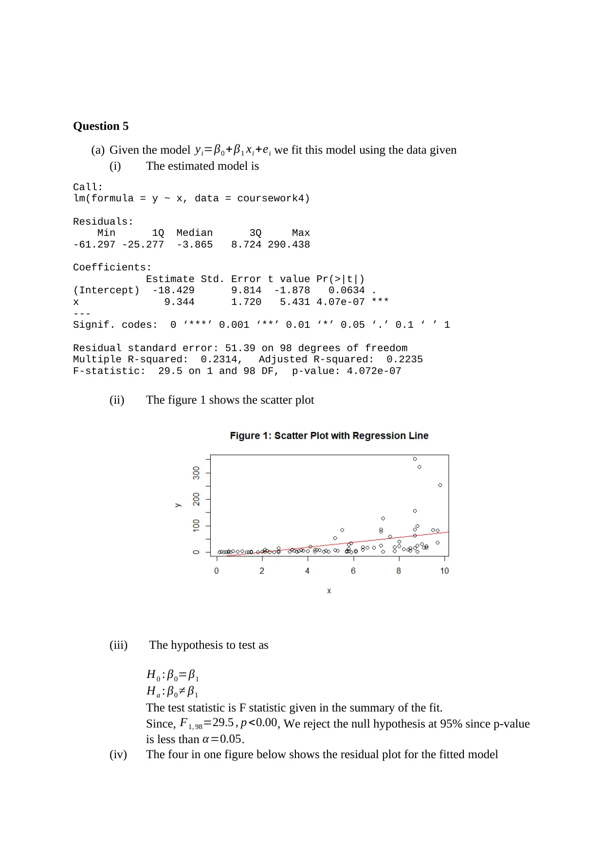
(a) Given the model yi=β0 + β1 xi +ei we fit this model using the data given
(i) The estimated model is
Call:
lm(formula = y ~ x, data = coursework4)
Residuals:
Min 1Q Median 3Q Max
-61.297 -25.277 -3.865 8.724 290.438
Coefficients:
Estimate Std. Error t value Pr(>|t|)
(Intercept) -18.429 9.814 -1.878 0.0634 .
x 9.344 1.720 5.431 4.07e-07 ***
---
Signif. codes: 0 ‘***’ 0.001 ‘**’ 0.01 ‘*’ 0.05 ‘.’ 0.1 ‘ ’ 1
Residual standard error: 51.39 on 98 degrees of freedom
Multiple R-squared: 0.2314, Adjusted R-squared: 0.2235
F-statistic: 29.5 on 1 and 98 DF, p-value: 4.072e-07
(ii) The figure 1 shows the scatter plot
(iii) The hypothesis to test as
H0 : β0=β1
Ha : β0 ≠ β1
The test statistic is F statistic given in the summary of the fit.
Since, F1, 98=29.5 , p <0.00, We reject the null hypothesis at 95% since p-value
is less than α =0.05.
(iv) The four in one figure below shows the residual plot for the fitted model

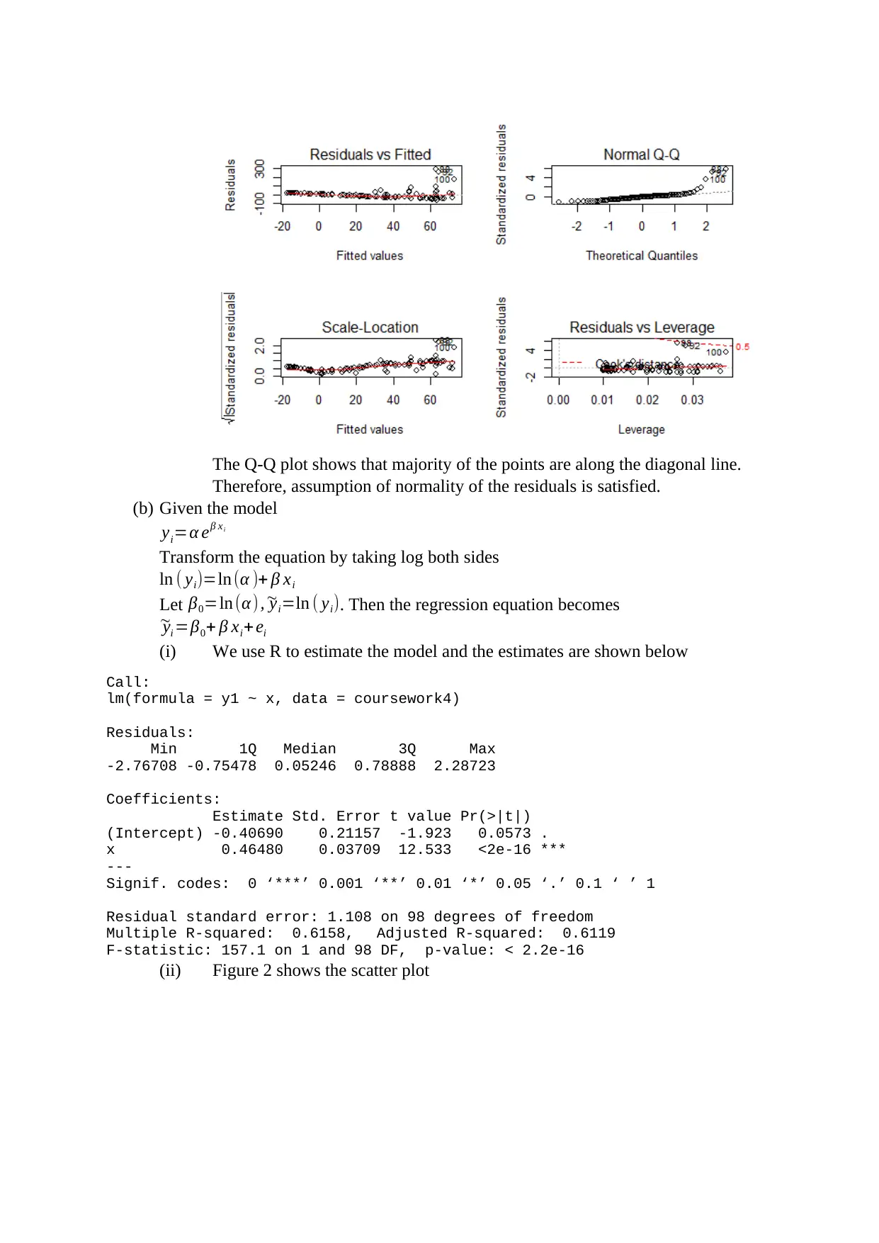
The Q-Q plot shows that majority of the points are along the diagonal line.
Therefore, assumption of normality of the residuals is satisfied.
(b) Given the model
yi=α eβ xi
Transform the equation by taking log both sides
ln ( yi)=ln (α )+ β xi
Let β0=ln (α ) , ~yi=ln ( yi). Then the regression equation becomes
~yi =β0+ β xi+ ei
(i) We use R to estimate the model and the estimates are shown below
Call:
lm(formula = y1 ~ x, data = coursework4)
Residuals:
Min 1Q Median 3Q Max
-2.76708 -0.75478 0.05246 0.78888 2.28723
Coefficients:
Estimate Std. Error t value Pr(>|t|)
(Intercept) -0.40690 0.21157 -1.923 0.0573 .
x 0.46480 0.03709 12.533 <2e-16 ***
---
Signif. codes: 0 ‘***’ 0.001 ‘**’ 0.01 ‘*’ 0.05 ‘.’ 0.1 ‘ ’ 1
Residual standard error: 1.108 on 98 degrees of freedom
Multiple R-squared: 0.6158, Adjusted R-squared: 0.6119
F-statistic: 157.1 on 1 and 98 DF, p-value: < 2.2e-16
(ii) Figure 2 shows the scatter plot

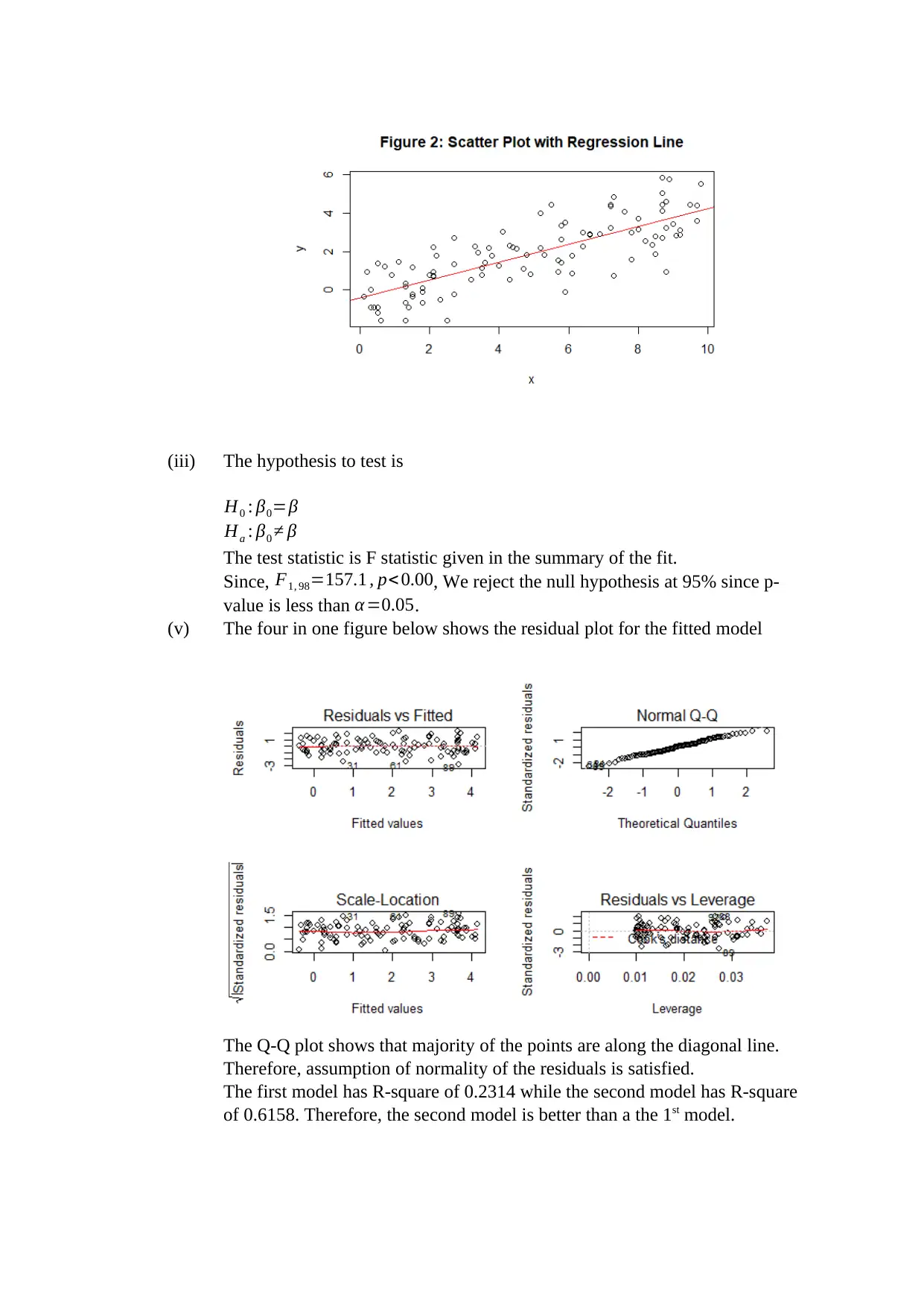
(iii) The hypothesis to test is
H0 : β0=β
Ha : β0 ≠ β
The test statistic is F statistic given in the summary of the fit.
Since, F1, 98=157.1 , p< 0.00, We reject the null hypothesis at 95% since p-
value is less than α =0.05.
(v) The four in one figure below shows the residual plot for the fitted model
The Q-Q plot shows that majority of the points are along the diagonal line.
Therefore, assumption of normality of the residuals is satisfied.
The first model has R-square of 0.2314 while the second model has R-square
of 0.6158. Therefore, the second model is better than a the 1st model.