Exploratory Data Analysis and Missing Data Analysis

This document provides an analysis of the data set including exploratory data analysis and missing data analysis. It also includes correlation and regression analysis.

Statistics
1

Part A.
1. Exploratory Data Analysis
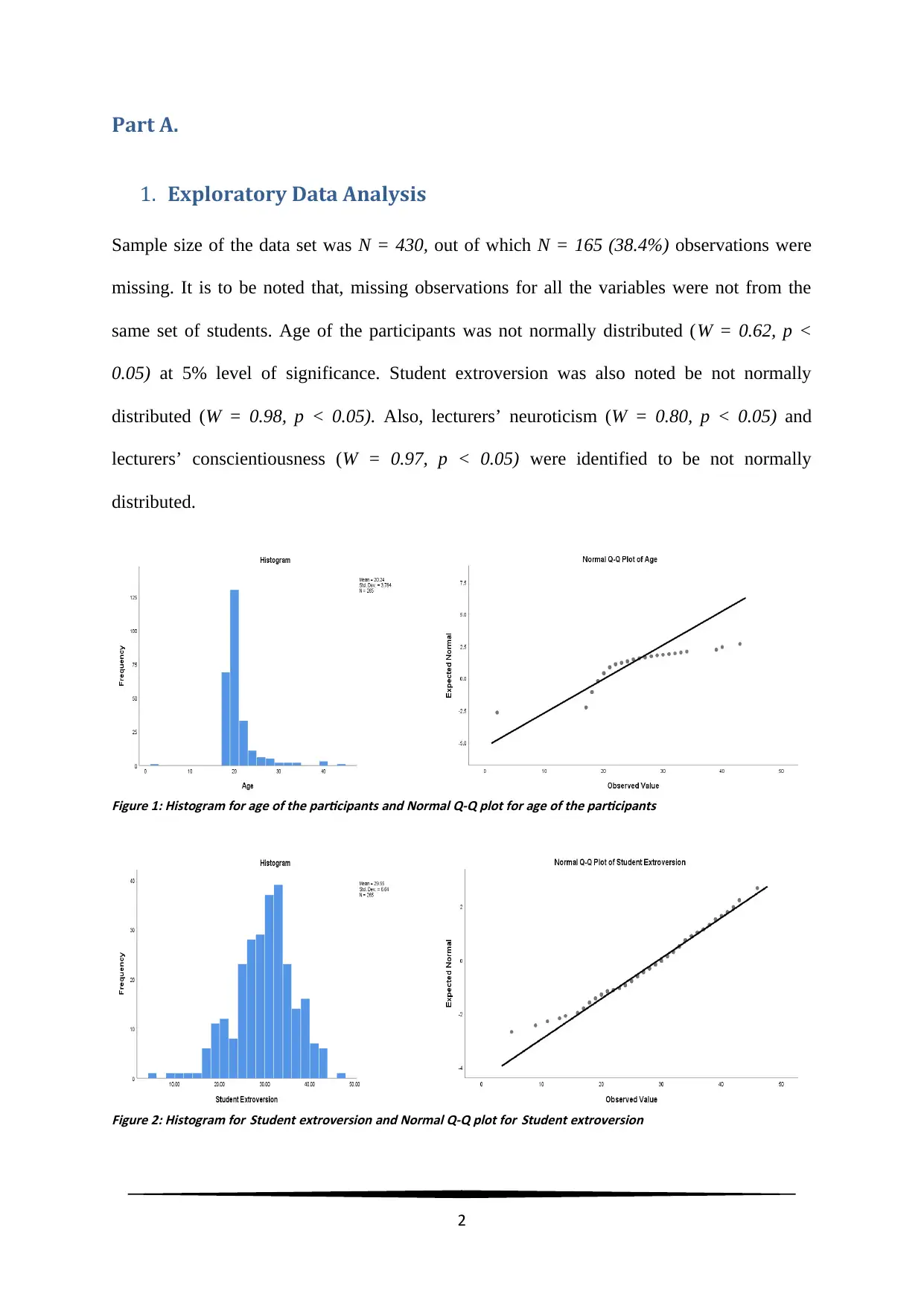
Sample size of the data set was N = 430, out of which N = 165 (38.4%) observations were
missing. It is to be noted that, missing observations for all the variables were not from the
same set of students. Age of the participants was not normally distributed (W = 0.62, p <
0.05) at 5% level of significance. Student extroversion was also noted be not normally
distributed (W = 0.98, p < 0.05). Also, lecturers’ neuroticism (W = 0.80, p < 0.05) and
lecturers’ conscientiousness (W = 0.97, p < 0.05) were identified to be not normally
distributed.
Figure 1: Histogram for age of the participants and Normal Q-Q plot for age of the participants
Figure 2: Histogram for Student extroversion and Normal Q-Q plot for Student extroversion
2

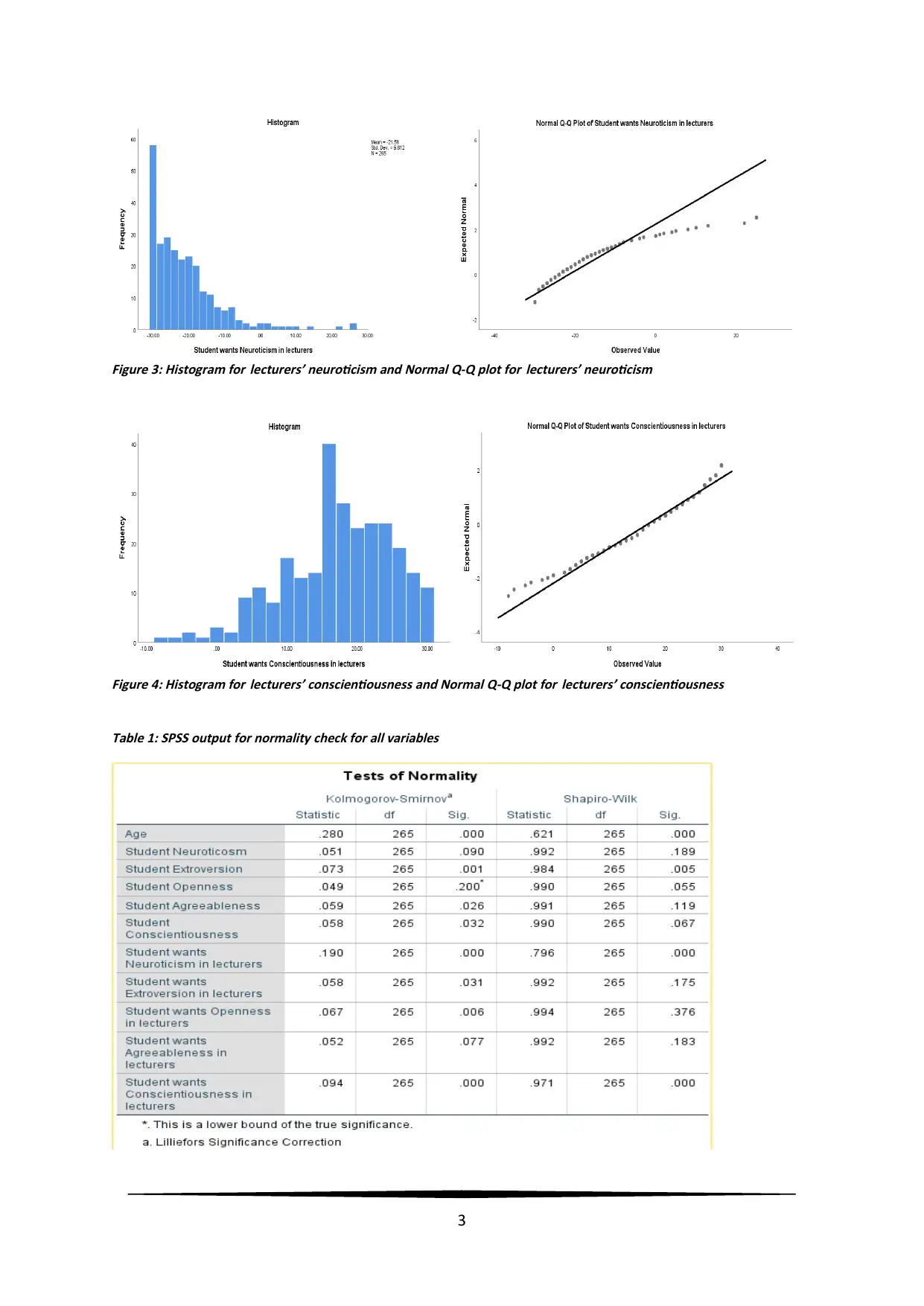
Figure 3: Histogram for lecturers’ neuroticism and Normal Q-Q plot for lecturers’ neuroticism
Figure 4: Histogram for lecturers’ conscientiousness and Normal Q-Q plot for lecturers’ conscientiousness
Table 1: SPSS output for normality check for all variables
3

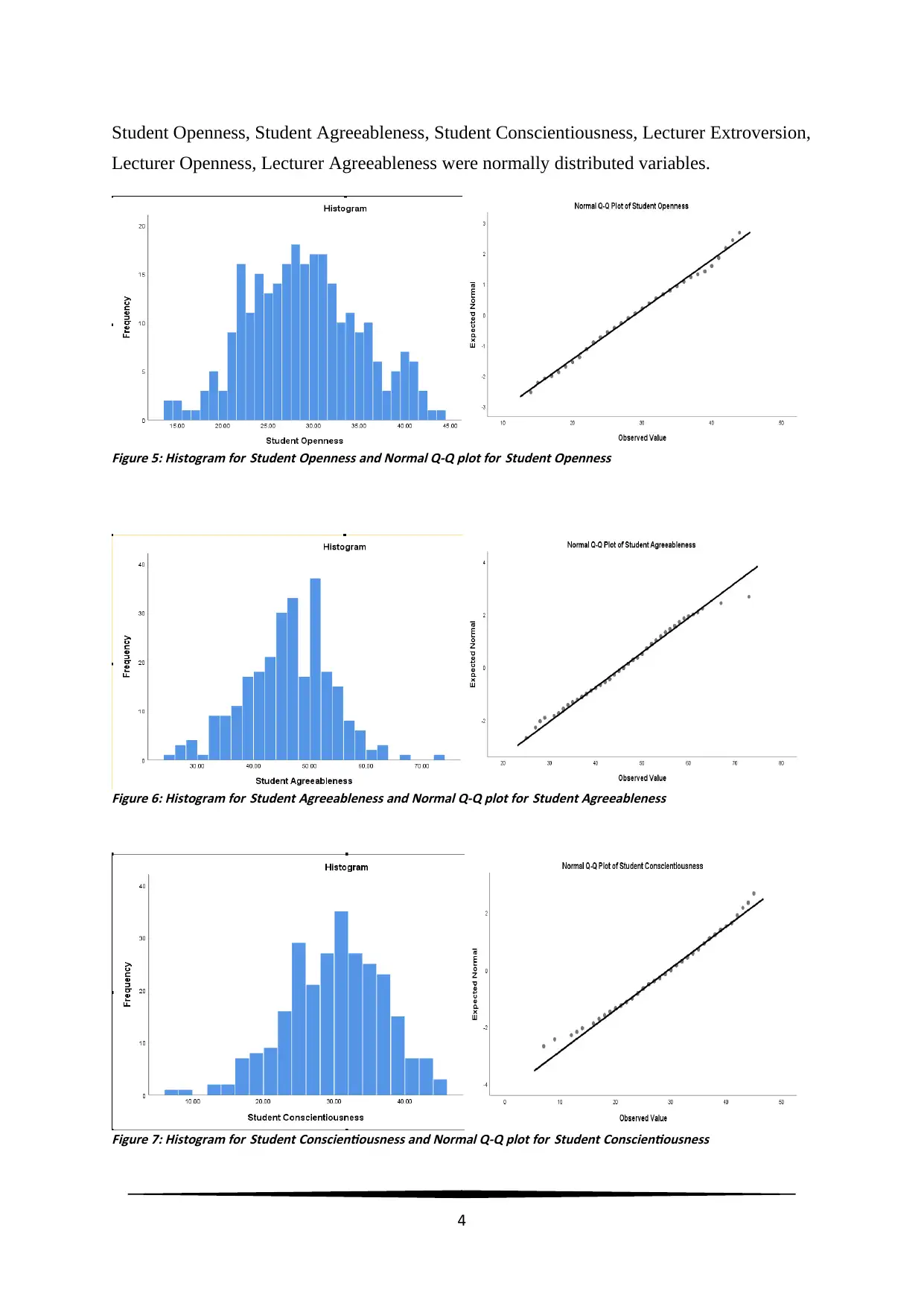
Student Openness, Student Agreeableness, Student Conscientiousness, Lecturer Extroversion,
Lecturer Openness, Lecturer Agreeableness were normally distributed variables.
Figure 5: Histogram for Student Openness and Normal Q-Q plot for Student Openness
Figure 6: Histogram for Student Agreeableness and Normal Q-Q plot for Student Agreeableness
Figure 7: Histogram for Student Conscientiousness and Normal Q-Q plot for Student Conscientiousness
4

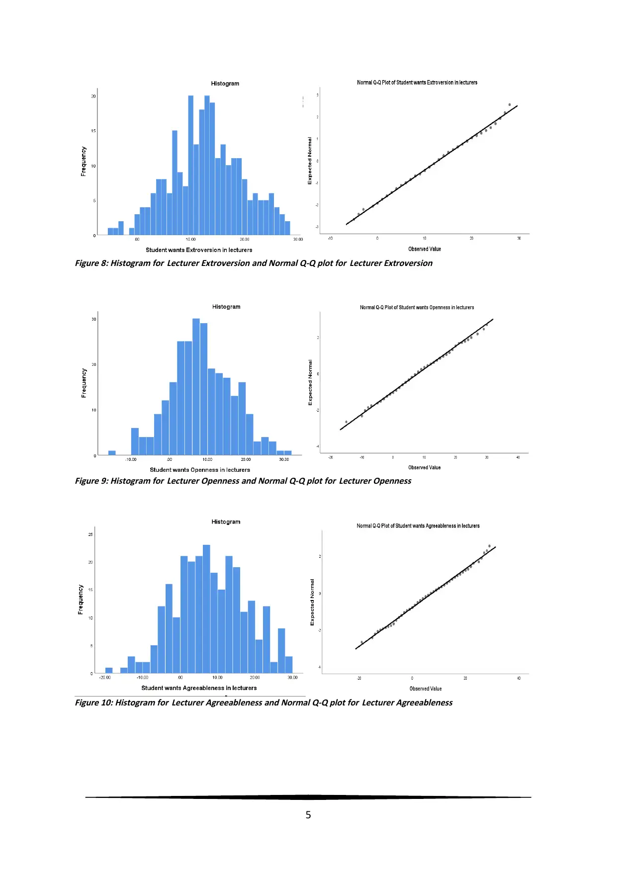
Figure 8: Histogram for Lecturer Extroversion and Normal Q-Q plot for Lecturer Extroversion
Figure 9: Histogram for Lecturer Openness and Normal Q-Q plot for Lecturer Openness
Figure 10: Histogram for Lecturer Agreeableness and Normal Q-Q plot for Lecturer Agreeableness
5

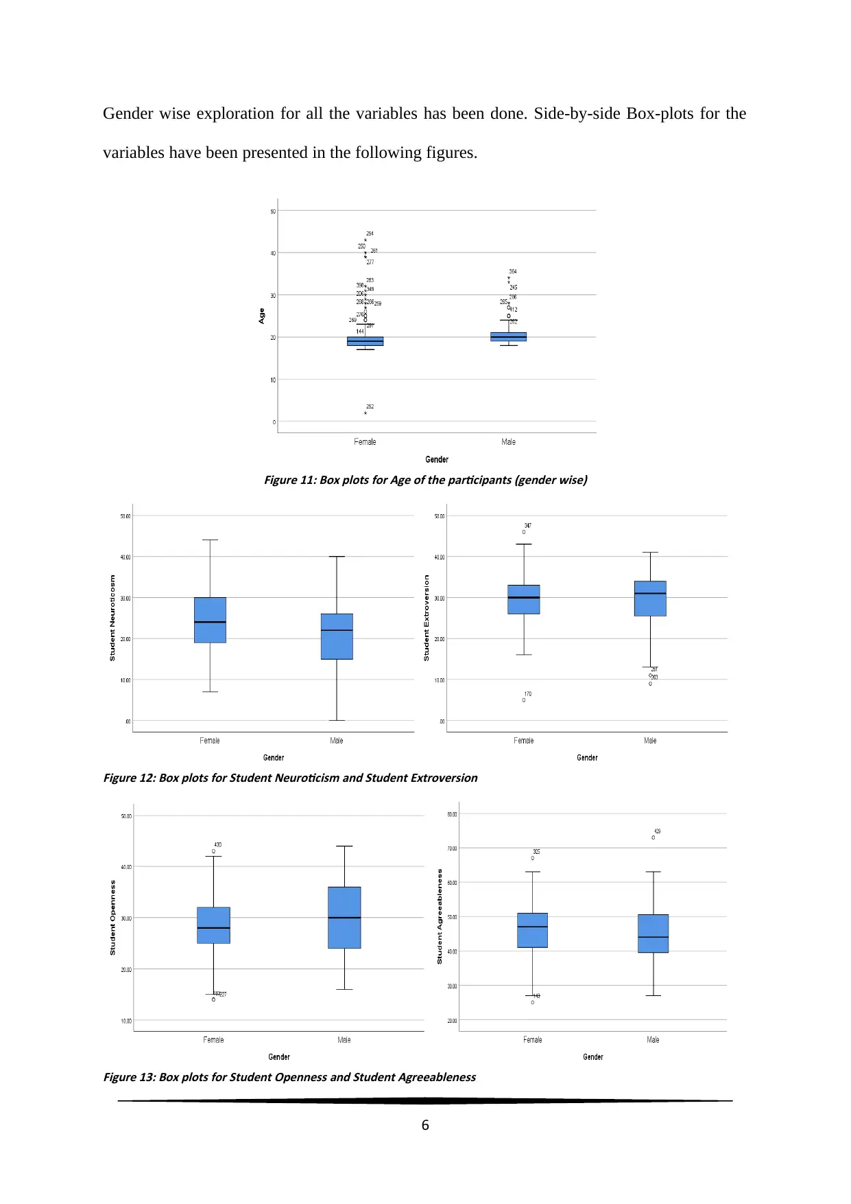
Gender wise exploration for all the variables has been done. Side-by-side Box-plots for the
variables have been presented in the following figures.
Figure 11: Box plots for Age of the participants (gender wise)
Figure 12: Box plots for Student Neuroticism and Student Extroversion
Figure 13: Box plots for Student Openness and Student Agreeableness
6

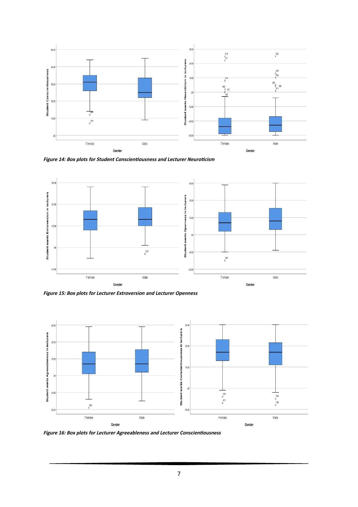
Figure 14: Box plots for Student Conscientiousness and Lecturer Neuroticism
Figure 15: Box plots for Lecturer Extroversion and Lecturer Openness
Figure 16: Box plots for Lecturer Agreeableness and Lecturer Conscientiousness
7

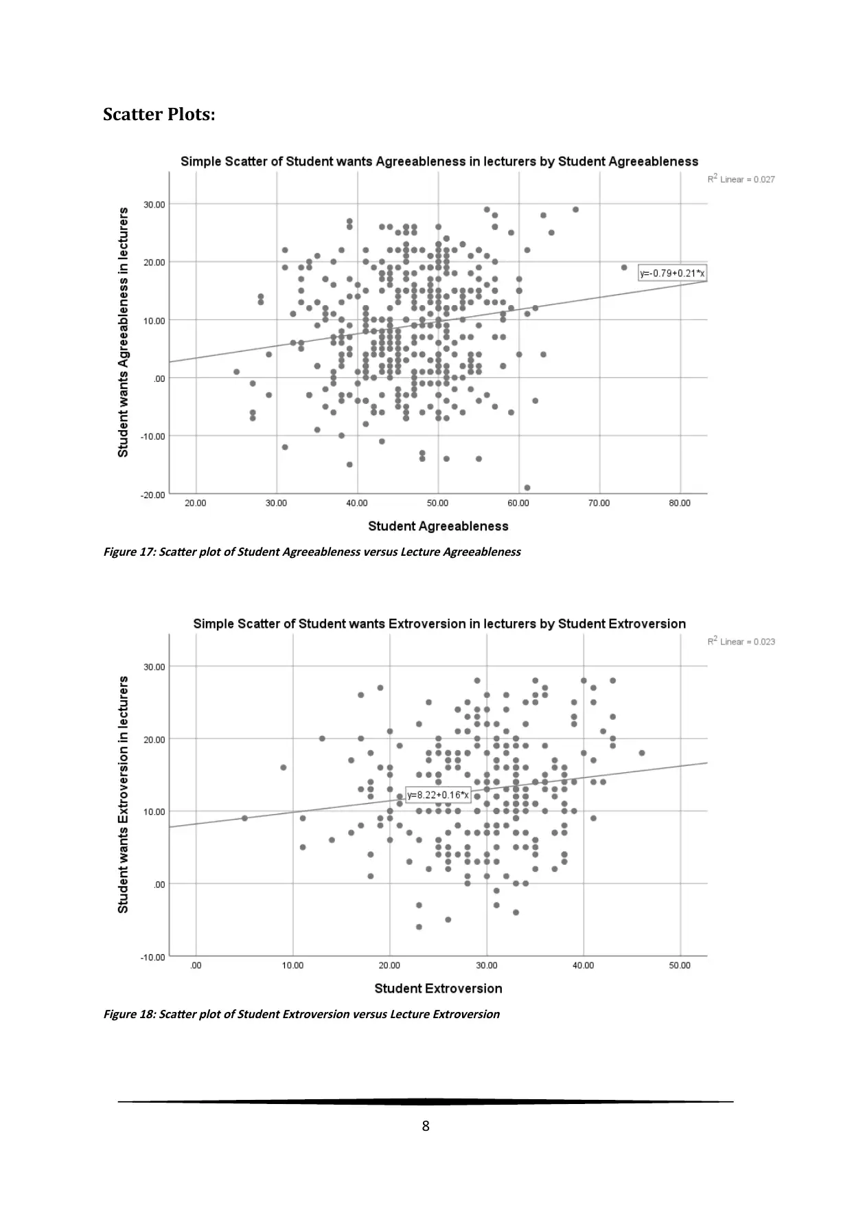
Scatter Plots:
Figure 17: Scatter plot of Student Agreeableness versus Lecture Agreeableness
Figure 18: Scatter plot of Student Extroversion versus Lecture Extroversion
8

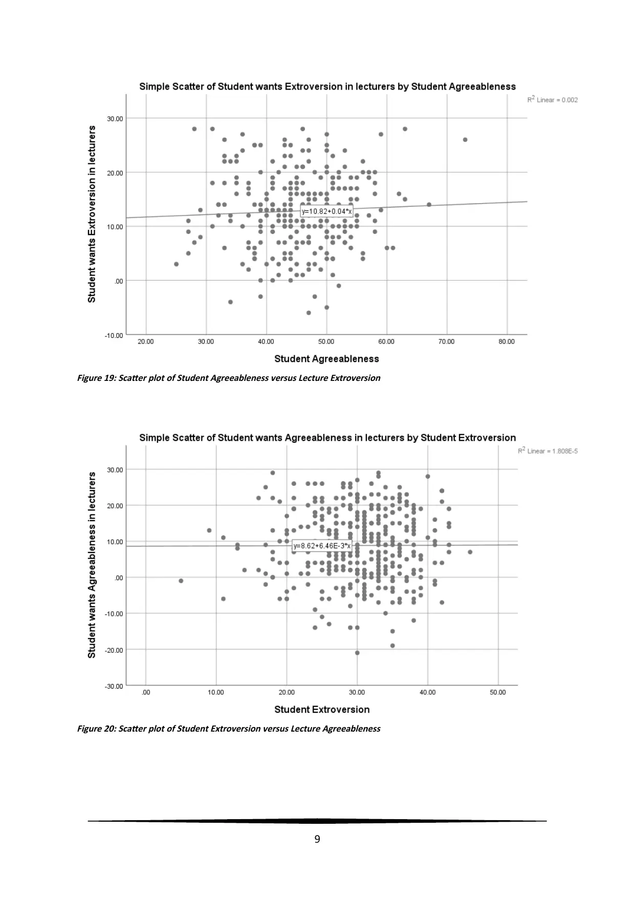
Figure 19: Scatter plot of Student Agreeableness versus Lecture Extroversion
Figure 20: Scatter plot of Student Extroversion versus Lecture Agreeableness
9

B. Description of the data
Total N = 430 responses were collected from the students. Gender wise exploration revealed
that 424 observations were valid, and gender information of rest 6 observations was missing.
Gender wise division reflected that female students (N =307, P 72.4%) were more than male
students in the sample (N =307, P 72.4%). Distribution of age of the participants was
affected by age of older participants (outliers). Age of the participants was not normally
distributed. Student extroversion, lecturers’ neuroticism, and lecturers’ conscientiousness
were identified to be not normally distributed variables.
From figure 11, Median age of males was noted be higher than that of the females. Presence
of extreme outliers was evident, especially for females. From figure 12, Student Neuroticism
was noted to be normally distributed for females, and little left skewed for males. Student
Extroversion for female students was almost normally distributed with few outliers, and left
skewed for males. From figure 13, Student Openness was noted to be normally distributed for
females (few outliers) and males. Student Extroversion was slightly left skewed for female
students, and almost normally distributed with few outliers for male students. From figure 14,
Student Conscientiousness was noted to be normally distributed for females (few outliers)
and highly right skewed for males. Lecturer Neuroticism was almost normal for females and
males with some extreme higher scores. From figure 15, Lecturer Extroversion was noted to
be normally distributed for females and slightly right skewed for males. Lecturer Openness
was almost normal for female and male students. From figure 16, Lecturer Agreeableness
was noted to be normally distributed for females and slightly right skewed for males.
Lecturer Conscientiousness was slight right for females with two outlier values, and little left
skewed for males. The scatter plots revealed low positive correlations between student
(Extroversion, Agreeableness) and lecturer (Extroversion, Agreeableness).
10

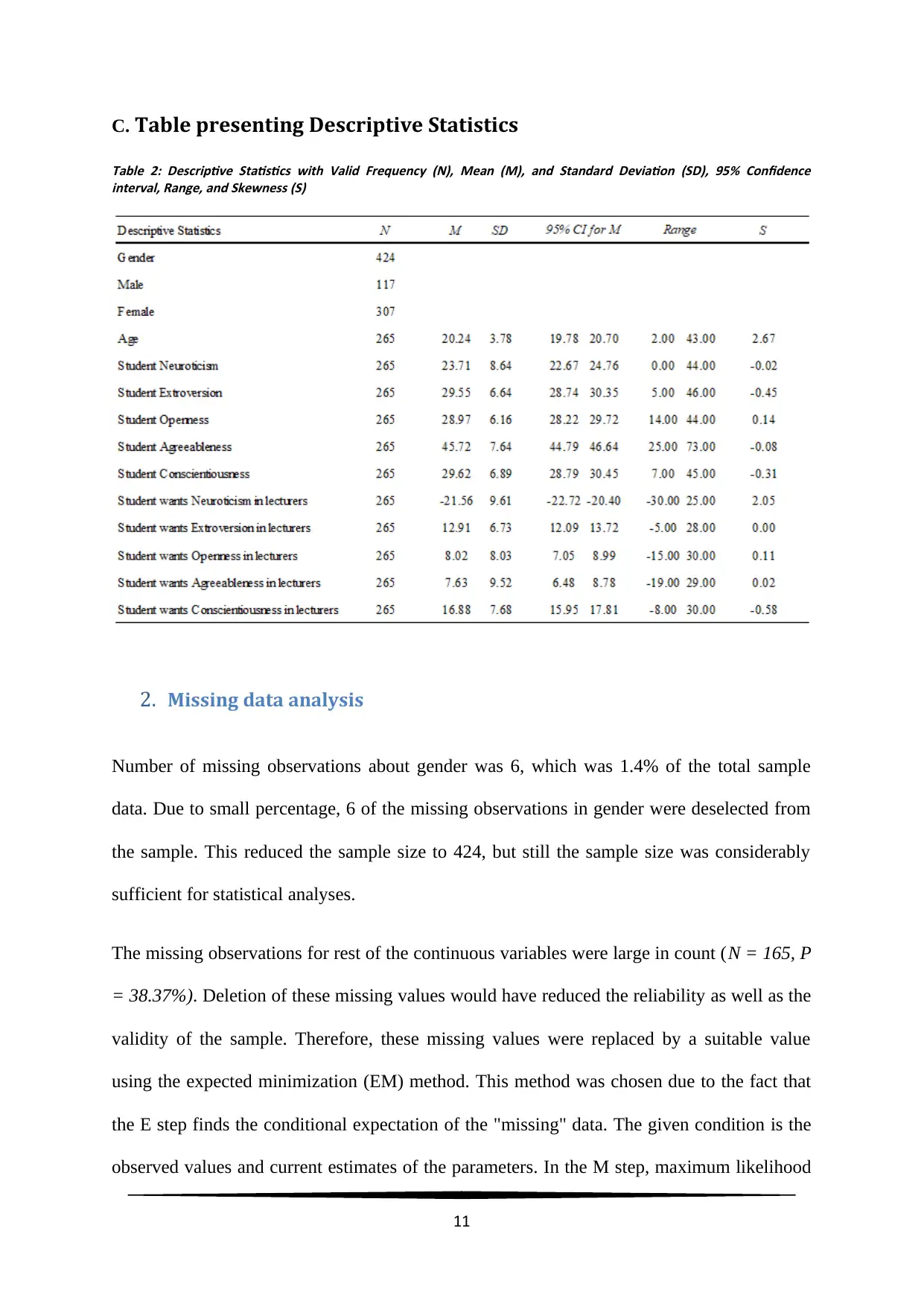
C. Table presenting Descriptive Statistics
Table 2: Descriptive Statistics with Valid Frequency (N), Mean (M), and Standard Deviation (SD), 95% Confidence
interval, Range, and Skewness (S)
2. Missing data analysis
Number of missing observations about gender was 6, which was 1.4% of the total sample
data. Due to small percentage, 6 of the missing observations in gender were deselected from
the sample. This reduced the sample size to 424, but still the sample size was considerably
sufficient for statistical analyses.
The missing observations for rest of the continuous variables were large in count (N = 165, P
= 38.37%). Deletion of these missing values would have reduced the reliability as well as the
validity of the sample. Therefore, these missing values were replaced by a suitable value
using the expected minimization (EM) method. This method was chosen due to the fact that
the E step finds the conditional expectation of the "missing" data. The given condition is the
observed values and current estimates of the parameters. In the M step, maximum likelihood
11

estimates of the parameters are calculated. As missing observations for all the variables were
not from the same set of students, EM method was best suited for treating the missing values.
3. Correlation
a. The missing observations were handled according to policies made in question 2.
b. One tail test has been used for finding the significance or p-values of the correlations. This
was due to the fact that the scatter diagrams indicated that there exist positive correlations
between the variables under examination.
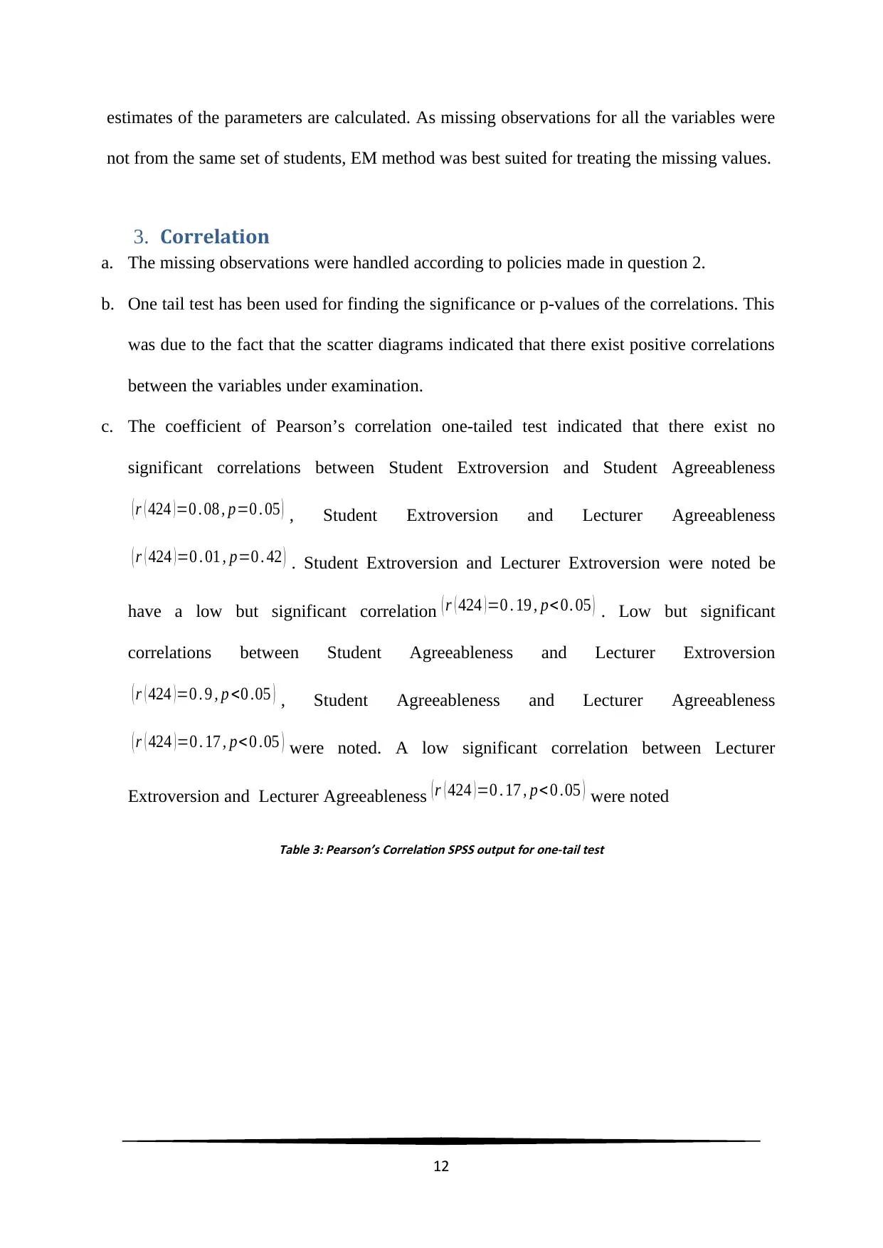
c. The coefficient of Pearson’s correlation one-tailed test indicated that there exist no
significant correlations between Student Extroversion and Student Agreeableness
( r ( 424 ) =0 . 08 , p=0 . 05 ) , Student Extroversion and Lecturer Agreeableness
( r ( 424 ) =0 . 01 , p=0 . 42 ) . Student Extroversion and Lecturer Extroversion were noted be
have a low but significant correlation ( r ( 424 ) =0 . 19 , p< 0. 05 ) . Low but significant
correlations between Student Agreeableness and Lecturer Extroversion
( r ( 424 ) =0 . 9 , p <0 .05 ) , Student Agreeableness and Lecturer Agreeableness
( r ( 424 ) =0 . 17 , p< 0 .05 ) were noted. A low significant correlation between Lecturer
Extroversion and Lecturer Agreeableness ( r ( 424 ) =0 . 17 , p< 0 .05 ) were noted
Table 3: Pearson’s Correlation SPSS output for one-tail test
12

4. Simple linear regression
a. The missing observations were handled according to policies made in question 2.
b. Two-tailed test was used for the simple linear regression model. Two-tailed test was
chosen for possible relationship with the independent variable in both directions
irrespective of direction of correlation between the variables.
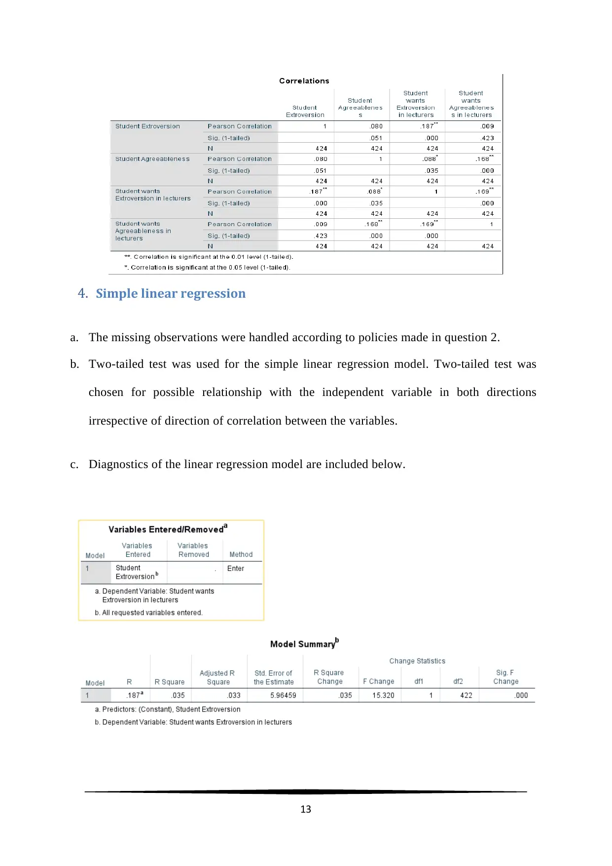
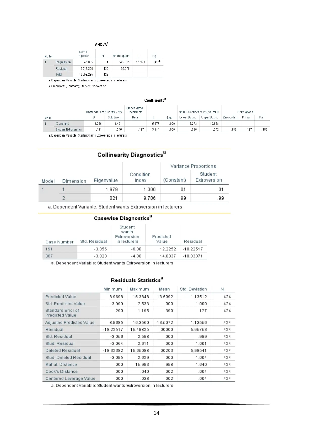
c. Diagnostics of the linear regression model are included below.
13

14

d. Assumptions:
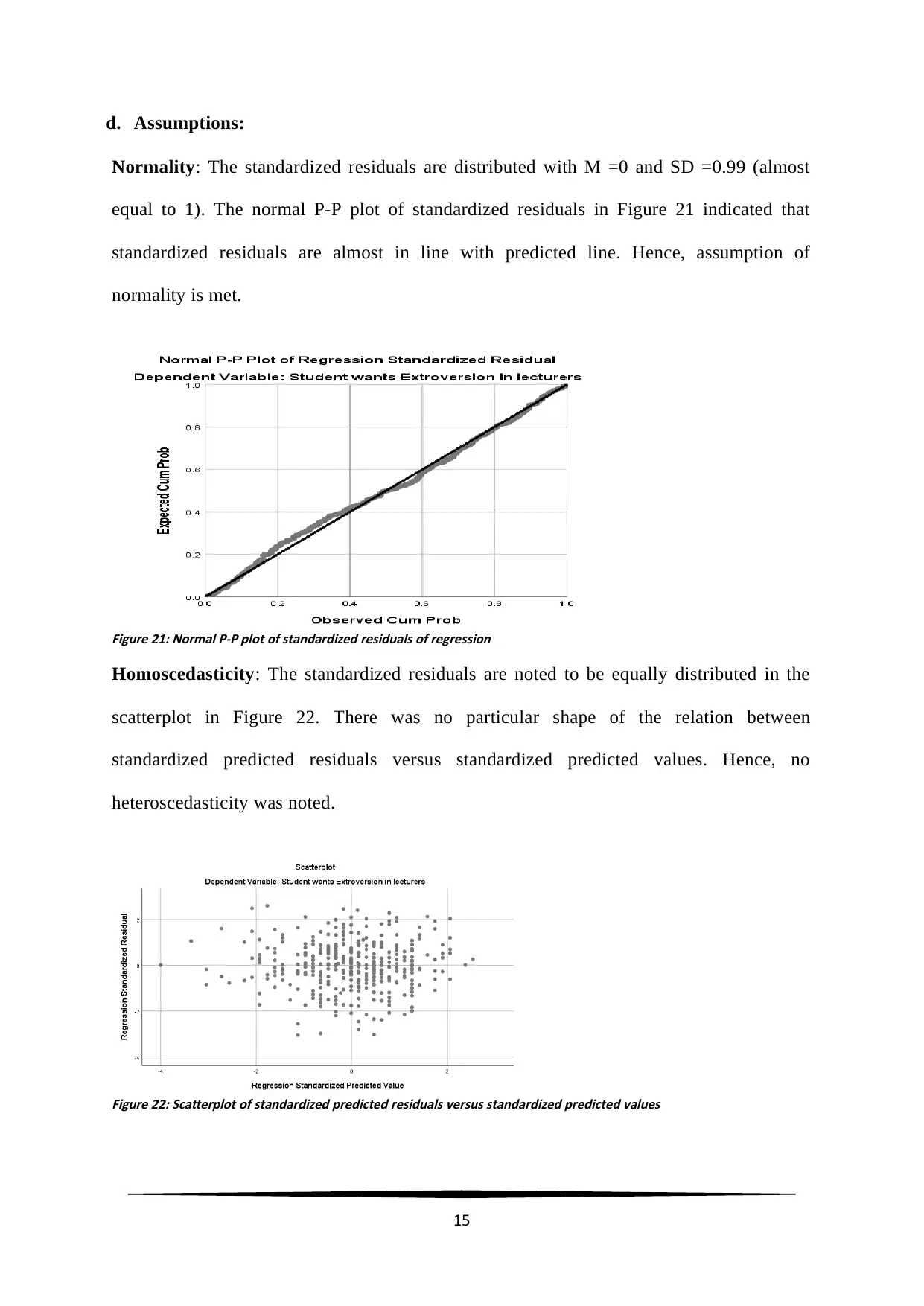
Normality: The standardized residuals are distributed with M =0 and SD =0.99 (almost
equal to 1). The normal P-P plot of standardized residuals in Figure 21 indicated that
standardized residuals are almost in line with predicted line. Hence, assumption of
normality is met.
Figure 21: Normal P-P plot of standardized residuals of regression
Homoscedasticity: The standardized residuals are noted to be equally distributed in the
scatterplot in Figure 22. There was no particular shape of the relation between
standardized predicted residuals versus standardized predicted values. Hence, no
heteroscedasticity was noted.
Figure 22: Scatterplot of standardized predicted residuals versus standardized predicted values
15

Linearity: The linear relation between lecturer extroversion and student’s extroversion
can be noted from the scatter plot in Figure 18, with positive correlation of 0.187.
Multicollinearity: There was no multicollinearity issue, as only single predictor was used.
Problems with outliers: The standard residuals ranged from -3.056 to 2.598. Case wise
diagnostics reflected that two of the cases with case numbers 191 and 387 had standard
residuals less than -3.0. Presence of these two outliers slightly reduced the correlation
between the variables.
e. A simple linear regression model has been used to predict Lecturer Extroversion based
on Student Extroversion. A significant regression equation was noted
( F ( 1 , 422 ) =15 . 32 , p<0 . 05 )
with coefficient of determination of
R2=0 . 035
. Predicted
Lecturer Extroversion is equal to
8 . 07+0 .18∗Student Extroversion
. Lecturer
Extroversion is noted to increase by 0.18 for each unit score of Student Extroversion.
f. The standardized beta coefficient was equal to the correlation coefficient. Therefore, the
regression results were in line with correlation result between Lecturer Extroversion and
Student Extroversion.
5. Multiple Regression
a. The missing observations were handled according to policies made in question 2.
b. Two-tailed test was used for the simple linear regression model. Two-tailed test was
chosen for possible relationship with the independent variable in both directions
irrespective of direction of correlation between the variables.
16

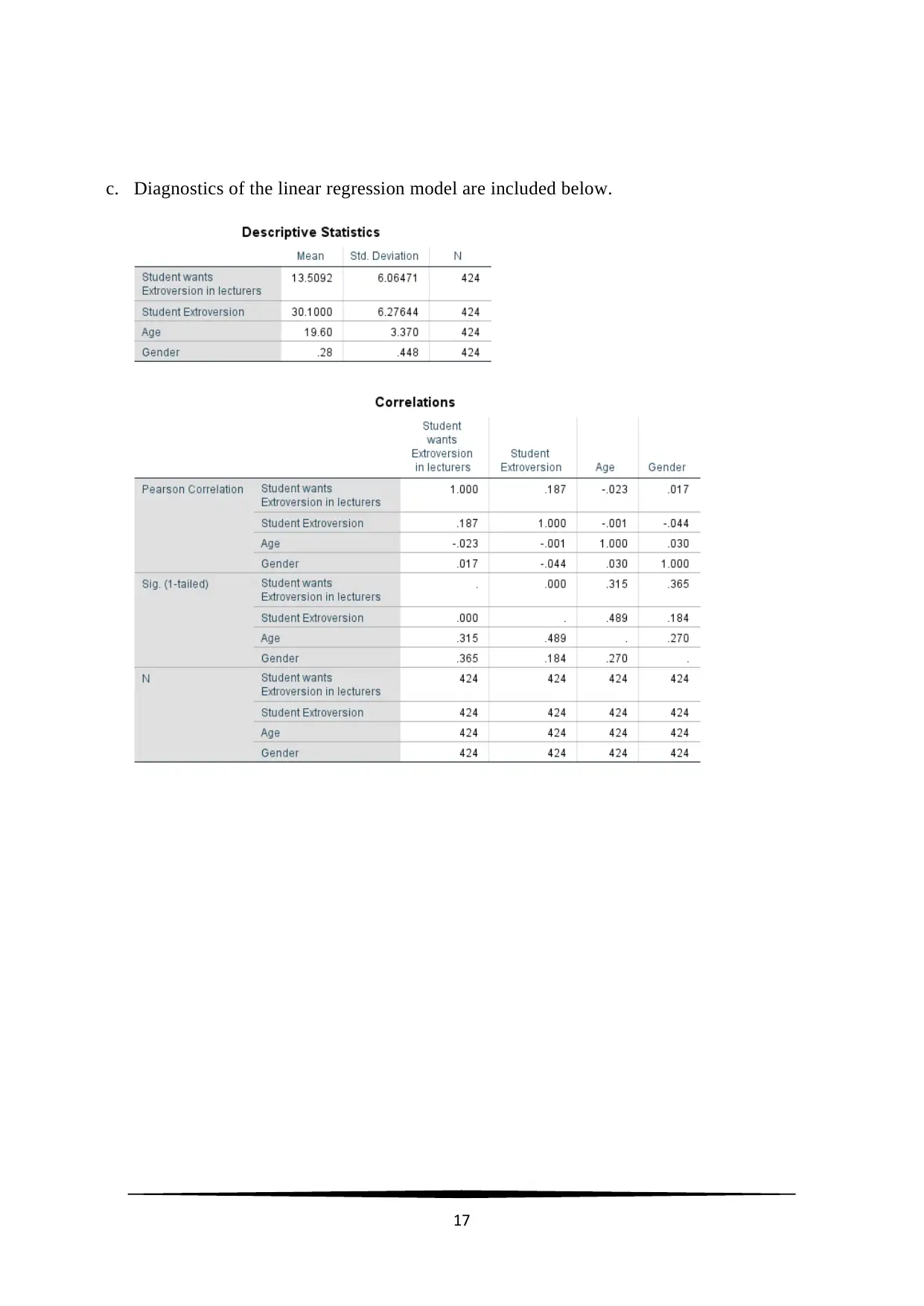
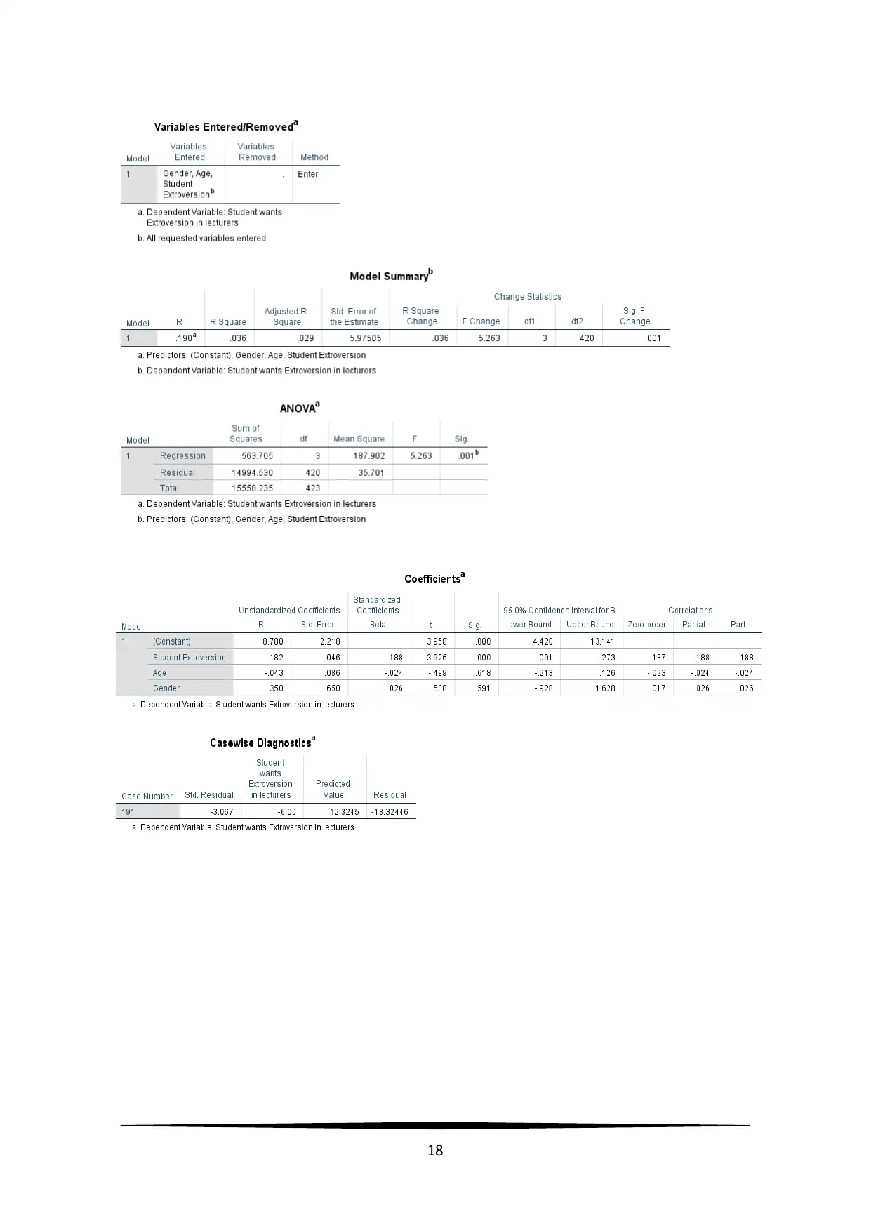
c. Diagnostics of the linear regression model are included below.
17

18

d. Assumptions:
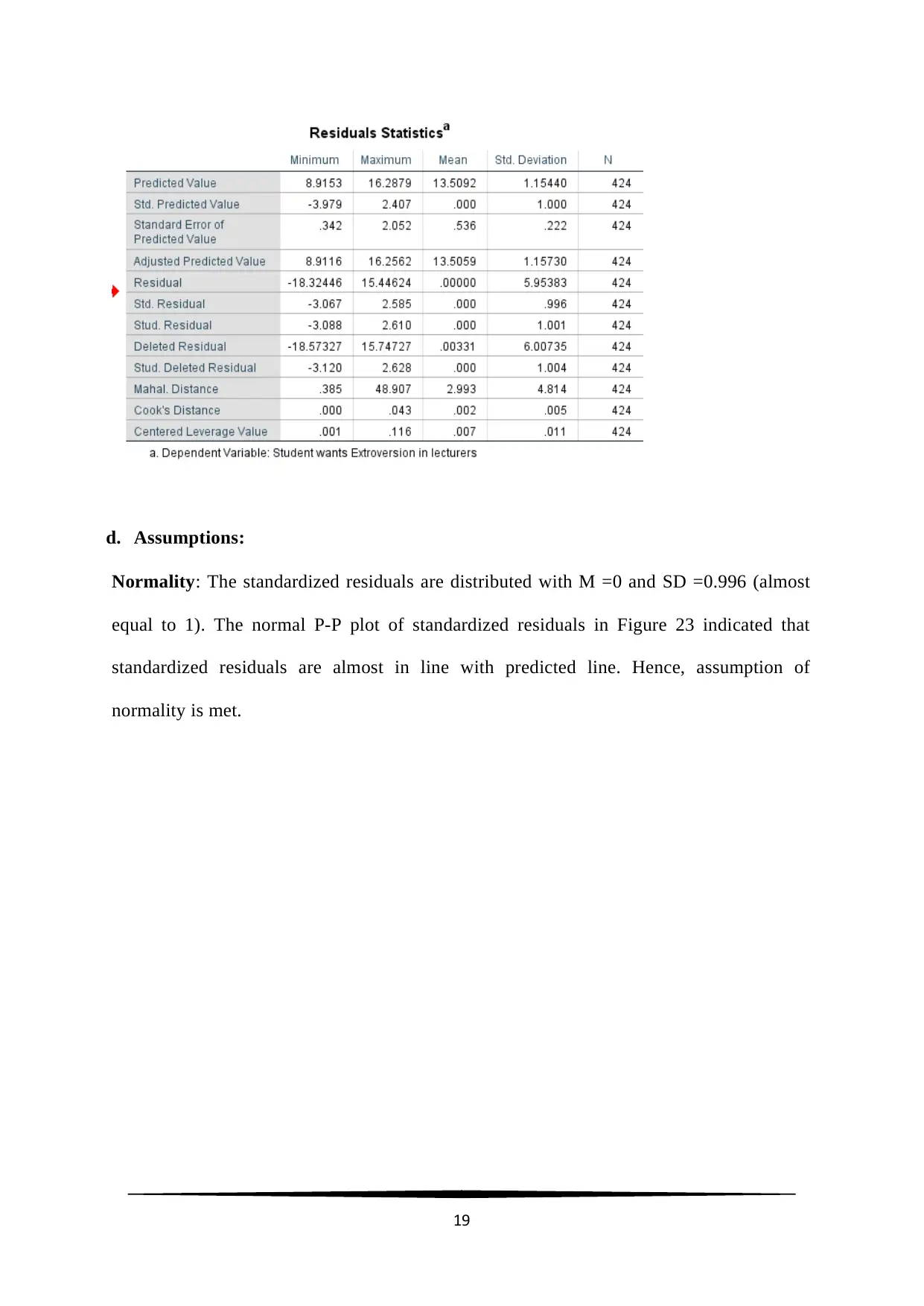
Normality: The standardized residuals are distributed with M =0 and SD =0.996 (almost
equal to 1). The normal P-P plot of standardized residuals in Figure 23 indicated that
standardized residuals are almost in line with predicted line. Hence, assumption of
normality is met.
19

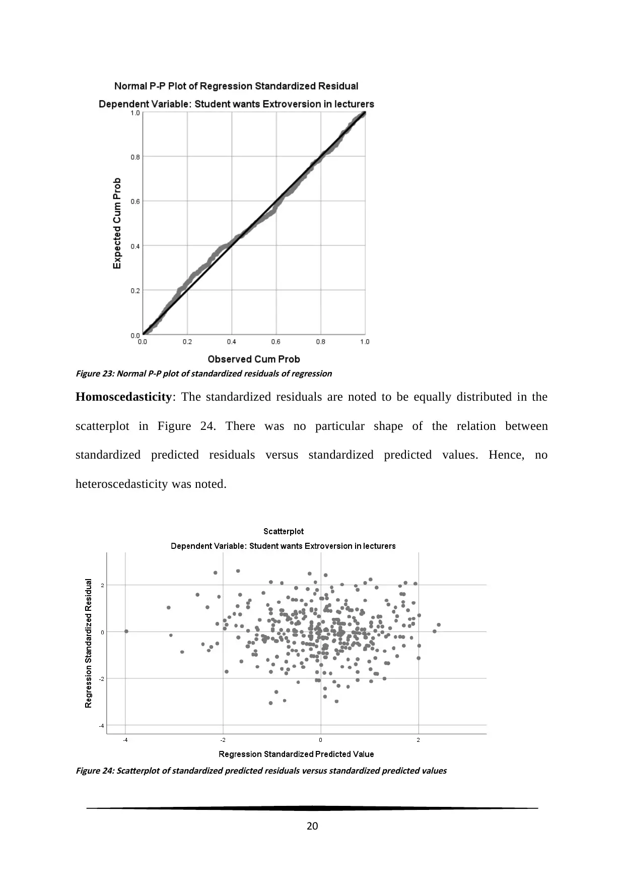
Figure 23: Normal P-P plot of standardized residuals of regression
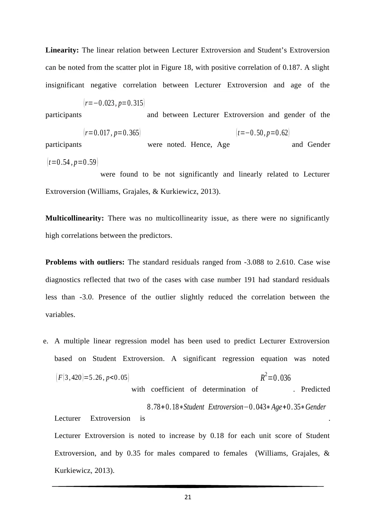
Homoscedasticity: The standardized residuals are noted to be equally distributed in the
scatterplot in Figure 24. There was no particular shape of the relation between
standardized predicted residuals versus standardized predicted values. Hence, no
heteroscedasticity was noted.
Figure 24: Scatterplot of standardized predicted residuals versus standardized predicted values
20

Linearity: The linear relation between Lecturer Extroversion and Student’s Extroversion
can be noted from the scatter plot in Figure 18, with positive correlation of 0.187. A slight
insignificant negative correlation between Lecturer Extroversion and age of the
participants
( r=−0 .023 , p=0. 315 )
and between Lecturer Extroversion and gender of the
participants
( r=0. 017 , p=0. 365 )
were noted. Hence, Age
( t=−0 . 50 , p=0 .62 )
and Gender
( t=0 .54 , p=0 .59 )
were found to be not significantly and linearly related to Lecturer
Extroversion (Williams, Grajales, & Kurkiewicz, 2013).
Multicollinearity: There was no multicollinearity issue, as there were no significantly
high correlations between the predictors.
Problems with outliers: The standard residuals ranged from -3.088 to 2.610. Case wise
diagnostics reflected that two of the cases with case number 191 had standard residuals
less than -3.0. Presence of the outlier slightly reduced the correlation between the
variables.
e. A multiple linear regression model has been used to predict Lecturer Extroversion
based on Student Extroversion. A significant regression equation was noted
( F ( 3 , 420 ) =5 .26 , p<0 . 05 )
with coefficient of determination of
R2=0 . 036
. Predicted
Lecturer Extroversion is
8 .78+ 0. 18∗Student Extroversion−0 . 043∗Age+0 . 35∗Gender
.
Lecturer Extroversion is noted to increase by 0.18 for each unit score of Student
Extroversion, and by 0.35 for males compared to females (Williams, Grajales, &
Kurkiewicz, 2013).
21

f. The regression results were in line with correlation results between Lecturer Extroversion
and Student Extroversion, Age, and Gender. The direction and significance of the
relations of correlations got preserved in the regression model.
Part B:
1. Area of research interest
Area of research is aimed to reconnoitre the linear relationship between the Miles per gallon
in city (MPG), Engine size, and Horsepower. Data will be collected through questionnaire
survey (Knittel, 2011).
a. Pearson Correlation
MPG and Horsepower are two selected variables, and the Pearson’s correlation coefficient
was calculated to find the linear association between the variables. Both MPG and
Horsepower are ratio scale variables. Pearson’s correlation coefficient was evaluated to be
( r=0. 42 , p<0 . 05 ) .
A positive and low effect size (Cohen) was noted with coefficient of determination as
R2=0 .176 . Now, this indicates that MPG and Horsepower were linearly related in positive
way, where Horsepower can explain 17.6% variation in MPG. Engine size was the third
variable which was linearly related to both MPG and Horsepower. Hence, Engine size, which
is the third variable, was the reason for this causal relationship.
b. Spearman’s Correlation
MPG and Horsepower are two selected variables, and the Spearman’s correlation coefficient,
due to high skewness of the variables, was calculated to find the linear association between
22

the variables. Both MPG and Horsepower are ratio scale variables. Spearman’s correlation
coefficient was evaluated to be ( r=0. 63 , p <0 . 05 ) .
A positive and moderate effect size (Cohen) was noted with coefficient of determination as
R2=0 .397 . Now, this indicates that MPG and Horsepower were linearly related in positive
way, where Horsepower can explain 39.7% variation in MPG. Engine size was the third
variable which was linearly related to both MPG and Horsepower. Hence, Engine size, which
is the third variable, was the reason for this causal relationship (de Winter, Gosling, & Potter,
2016).
c. Partial Correlation vs. Semi-Partial Correlation
Horsepower, Engine size, and Miles per gallon (MPG) are three selected variables for which
partial correlations, (bivariate correlation with accounting for relation with other variables)
and semi-partial correlations were found.
The partial correlation will hold constant the third variable by means of residuals. With
partial correlation, one can find the correlation between Horsepower and Miles per gallon
(MPG) holding Engine size constant for both Horsepower and Miles per gallon (MPG).
Sometimes, one can want to hold Engine size constant for just Horsepower or just MPG.
Therefore, this is called a semi-partial correlation instead of a partial. With a semi-partial,
we find the residuals of Horsepower on Engine size or MPG on Engine size but the other is
the original variable. Here the correlation is between one original and one residual.
Therefore, to assess the individual impact of Engine size and Horsepower on Miles per
gallon, semi-partial correlation will be the better choice.
d. Simple Regression
23

Horsepower and Miles per gallon (MPG) are the selected variables for simple regression.
Both variables are ratio scale variables. Horsepower will be the predictor and Miles per
gallon (MPG) will be the outcome variable. People are generally interested in MPG of a car,
and Horsepower has a causal relationship with it. The coefficient of determination ( R2 ) will
tell the percentage of proportion of the variance in MPG that is predictable from Horsepower.
e. Multiple Regression
Engine size, Horsepower and Miles per gallon (MPG) are the selected variables for multiple
regression analysis. All the variables are ratio scale variables. Engine size and Horsepower
will be the predictors and Miles per gallon (MPG) will be the outcome variable. The reason is
that the people are generally interested in MPG of a car, Engine Size and Horsepower have a
causal relationship with it. The coefficient of determination ( R2 ) will tell the percentage of
proportion of the variance in MPG that is predictable from Engine size and Horsepower. R2
assumed that Engine size and Horsepower explain the change to MPG. Adjusted R2 gave the
percentage change that is explained only by Engine size and Horsepower that actually affect
the MPG (Hidalgo, & Goodman, 2013).
f. Logistic Regression
Engine size, Horsepower and Miles per gallon (MPG) (Now, dichotomous in nature) are the
selected variables for multiple regression analysis. Engine size and Horsepower are ratio
scale variables. Miles per gallon has two outcomes and is a binary variable. “Good” (MPG
greater than or equal to 60) and “Bad” (MPG less than 60) are two dichotomous outcomes.
Engine size and Horsepower will be the predictors and Miles per gallon (MPG) will be the
outcome variable. The reason is that the people are generally interested in MPG of a car,
Engine Size and Horsepower have a causal relationship with it. Logit regression or Binary
logistic regression will be the regression modelling. The coefficient for Engine size says that,
24

holding Horsepower at a fixed value, we will see 13% increase in the odds of becoming a
Good MPG vehicle class for a one-unit increase in Engine size since exp(.12296) = 1.13
(values have been mocked).
References
de Winter, J. C., Gosling, S. D., & Potter, J. (2016). Comparing the Pearson and Spearman
correlation coefficients across distributions and sample sizes: A tutorial using
simulations and empirical data. Psychological methods, 21(3), 273.
Hidalgo, B., & Goodman, M. (2013). Multivariate or multivariable regression?. American
journal of public health, 103(1), 39-40.
Knittel, C. R. (2011). Automobiles on steroids: Product attribute trade-offs and technological
progress in the automobile sector. American Economic Review, 101(7), 3368-99.
Ngo, T. H. D., & La Puente, C. A. (2012, April). The steps to follow in a multiple regression
analysis. In Proceedings of the SAS Global Forum (pp. 22-25).
Williams, M. N., Grajales, C. A. G., & Kurkiewicz, D. (2013). Assumptions of multiple
regression: Correcting two misconceptions.
25