Calculating Confidence Interval for Change Support & Work-Life Balance Analysis

This assignment involves two main tasks: first, calculate the 95% confidence interval for the proportion of respondents supporting change (mean = 0.6, sample size = 112, SD = 0.0357). Second, analyze a work-life balance survey dataset containing 20 responses with gender and work-life balance status as variables. Use pivot tables to summarize categorical data, and interpret results.

Statistics

TABLE OF CONTENTS
SECTION 1.....................................................................................................................................1
a. Presenting scatter plot on the basis of given data set...............................................................1
b. Estimating annual contribution if income is $200,000............................................................1
c. Finding Z score........................................................................................................................1
d. Assessing P(Z < zscore)...........................................................................................................2
e. Ranking....................................................................................................................................2
SECTION 2.....................................................................................................................................3
a. Pivot table by using excel........................................................................................................3
b. Graphical presentation.............................................................................................................4
c. Commenting on the relationship takes place between the two variables.................................4
d...................................................................................................................................................4
1. Stating the deviations take place in the sample proportion.....................................................4
2. Assessing the value of Z score.................................................................................................4
3. Determining P(Z<zscore)........................................................................................................5
4. Give ranking on the basis of estimation..................................................................................5
e. Testing there is a difference in the proportions @ 5% level of significance...........................6
1. Stating hypothesis....................................................................................................................6
2. Finding p value........................................................................................................................6
3. Stating whether null hypothesis is true or false.......................................................................7
4. Conclusion...............................................................................................................................8
SECTION 3.....................................................................................................................................8
a. Creating a pivot table for summarizing statistical information...............................................8
b. Creating appropriate graph to show the relationship between the variables...........................8
c. Commenting on the relationship between the variables..........................................................9

d...................................................................................................................................................9
1. Difference between the sample means x 1-x 2.........................................................................9
2. Z-score.....................................................................................................................................9
3.................................................................................................................................................10
4.................................................................................................................................................10
e. Testing significant differences in the mean value @ 5% level of significance.....................11
1. Hypothesis.............................................................................................................................11
2.................................................................................................................................................11
3.................................................................................................................................................11
4.................................................................................................................................................11
SECTION 4...................................................................................................................................12
a..................................................................................................................................................12
b.................................................................................................................................................12
c. Assessing Z score...................................................................................................................12
1.................................................................................................................................................12
2.................................................................................................................................................12
3. Ranking..................................................................................................................................13
d. Finding 95% confidence interval level for the people who support change..........................13
SECTION 5...................................................................................................................................14
A and c Creating or obtaining own data set...............................................................................14
b. Summarizing variables by using pivot table..........................................................................14
SECTION 6...................................................................................................................................15
Discussing the manner in which mean and standard deviations are used in finance.................15

SECTION 1
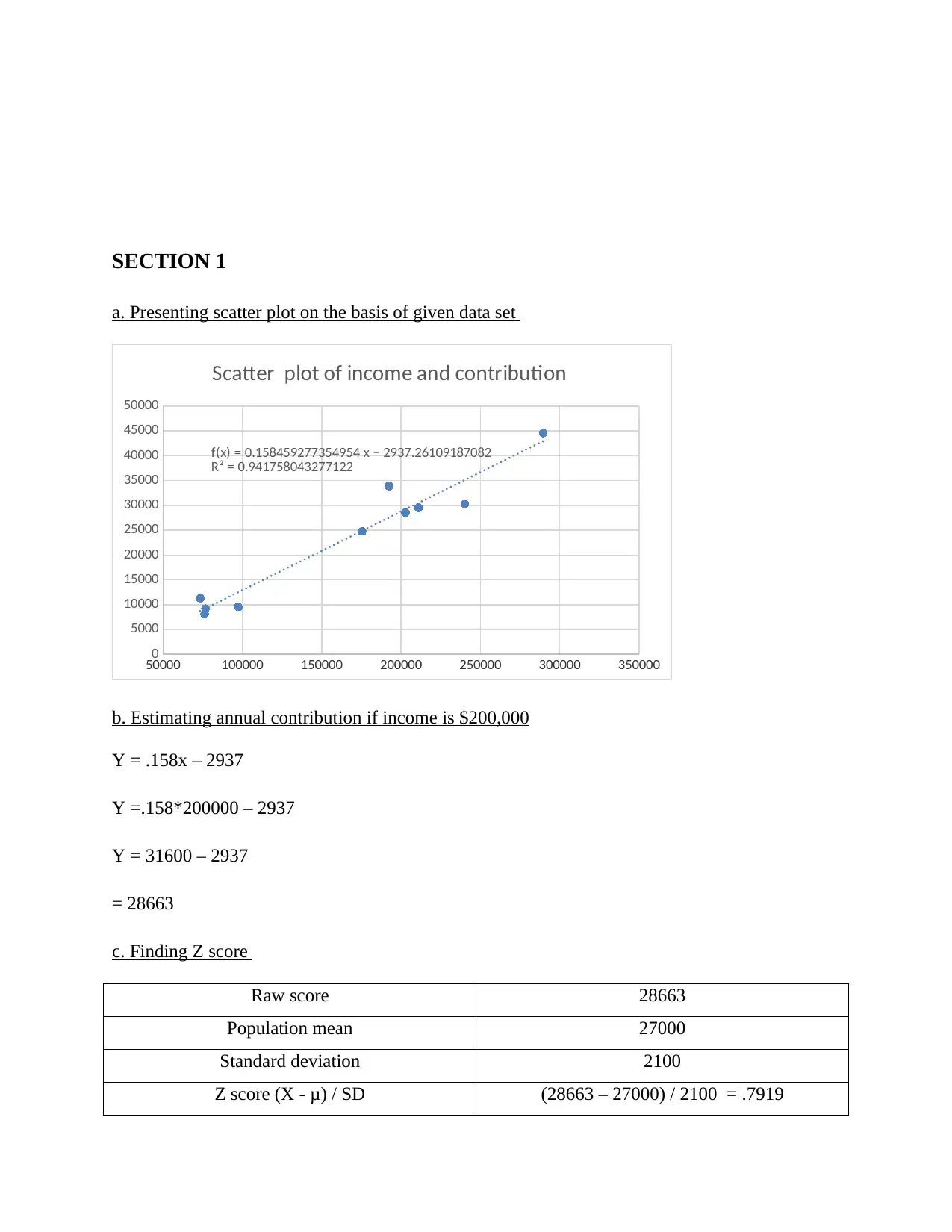
a. Presenting scatter plot on the basis of given data set
50000 100000 150000 200000 250000 300000 350000
0
5000
10000
15000
20000
25000
30000
35000
40000
45000
50000
f(x) = 0.158459277354954 x − 2937.26109187082
R² = 0.941758043277122
Scatter plot of income and contribution
b. Estimating annual contribution if income is $200,000
Y = .158x – 2937
Y =.158*200000 – 2937
Y = 31600 – 2937
= 28663
c. Finding Z score
Raw score 28663
Population mean 27000
Standard deviation 2100
Z score (X - μ) / SD (28663 – 27000) / 2100 = .7919

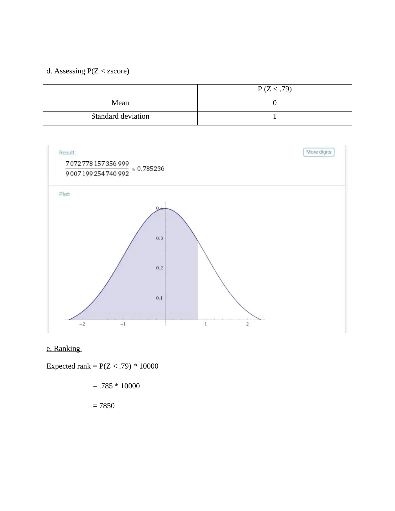
d. Assessing P(Z < zscore)
P (Z < .79)
Mean 0
Standard deviation 1
e. Ranking
Expected rank = P(Z < .79) * 10000
= .785 * 10000
= 7850

SECTION 2
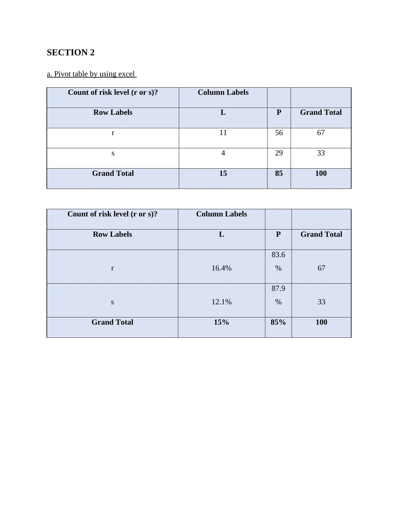
a. Pivot table by using excel
Count of risk level (r or s)? Column Labels
Row Labels L P Grand Total
r 11 56 67
s 4 29 33
Grand Total 15 85 100
Count of risk level (r or s)? Column Labels
Row Labels L P Grand Total
r 16.4%
83.6
% 67
s 12.1%
87.9
% 33
Grand Total 15% 85% 100

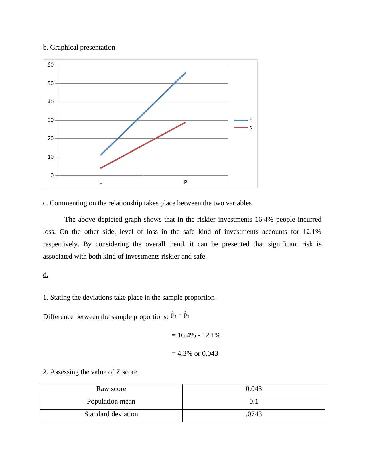
b. Graphical presentation
L P
0
10
20
30
40
50
60
r
s
c. Commenting on the relationship takes place between the two variables
The above depicted graph shows that in the riskier investments 16.4% people incurred
loss. On the other side, level of loss in the safe kind of investments accounts for 12.1%
respectively. By considering the overall trend, it can be presented that significant risk is
associated with both kind of investments riskier and safe.
d.
1. Stating the deviations take place in the sample proportion
Difference between the sample proportions:
= 16.4% - 12.1%
= 4.3% or 0.043
2. Assessing the value of Z score
Raw score 0.043
Population mean 0.1
Standard deviation .0743

Z score (X - μ) / SD (.043 – 0.1) / .0743 = -0.76716
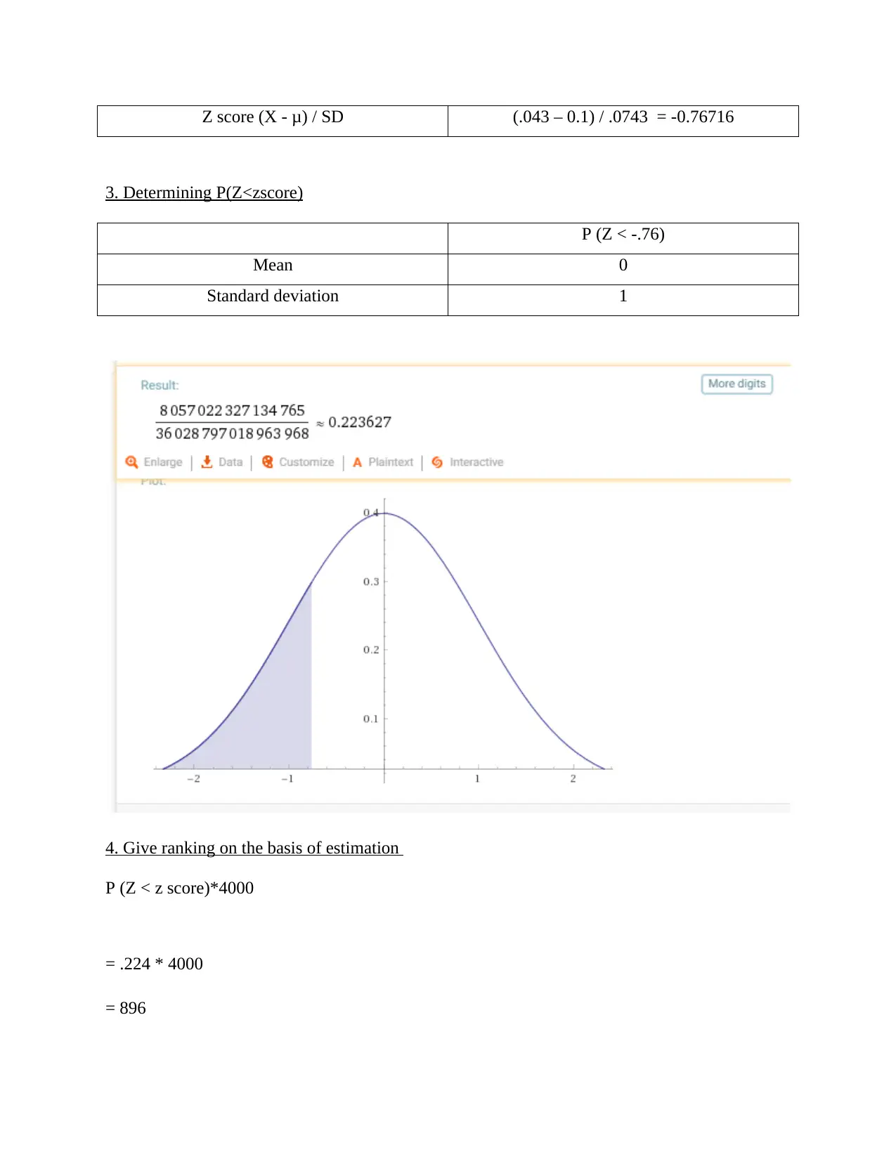
3. Determining P(Z<zscore)
P (Z < -.76)
Mean 0
Standard deviation 1
4. Give ranking on the basis of estimation
P (Z < z score)*4000
= .224 * 4000
= 896

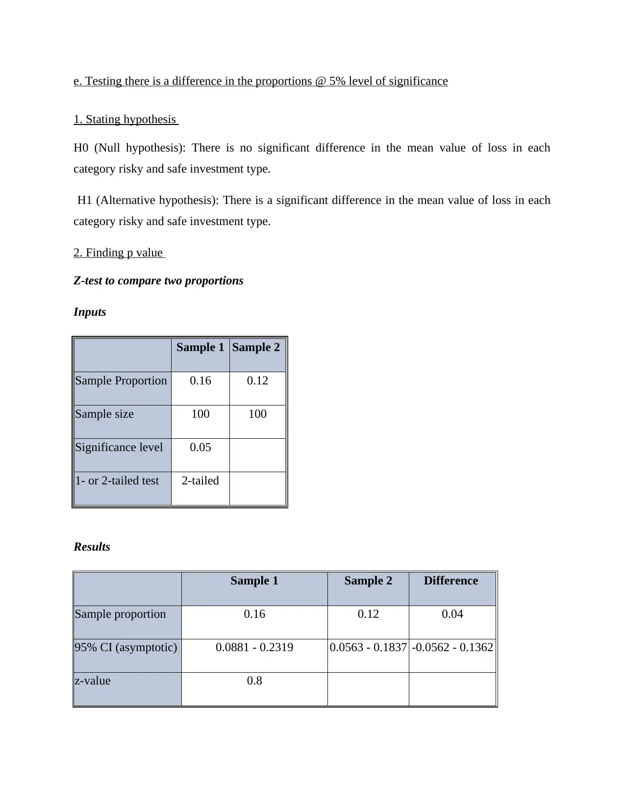
e. Testing there is a difference in the proportions @ 5% level of significance
1. Stating hypothesis
H0 (Null hypothesis): There is no significant difference in the mean value of loss in each
category risky and safe investment type.
H1 (Alternative hypothesis): There is a significant difference in the mean value of loss in each
category risky and safe investment type.
2. Finding p value
Z-test to compare two proportions
Inputs
Sample 1 Sample 2
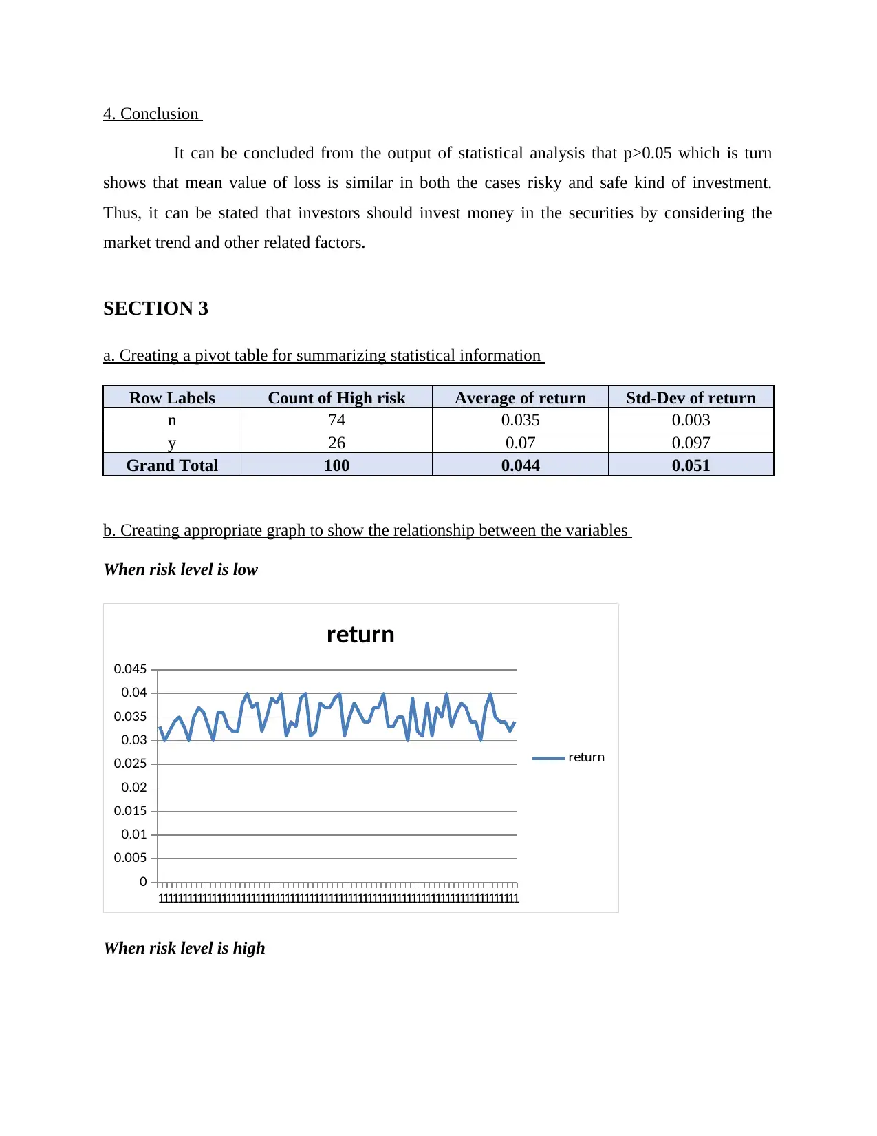
Sample Proportion 0.16 0.12
Sample size 100 100
Significance level 0.05
1- or 2-tailed test 2-tailed
Results
Sample 1 Sample 2 Difference
Sample proportion 0.16 0.12 0.04
95% CI (asymptotic) 0.0881 - 0.2319 0.0563 - 0.1837 -0.0562 - 0.1362
z-value 0.8

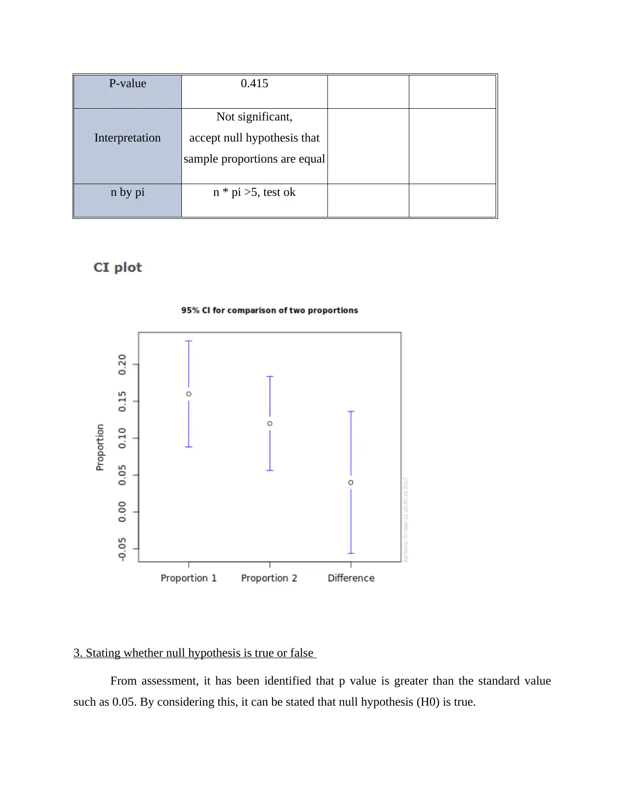
P-value 0.415
Interpretation
Not significant,
accept null hypothesis that
sample proportions are equal
n by pi n * pi >5, test ok
3. Stating whether null hypothesis is true or false
From assessment, it has been identified that p value is greater than the standard value
such as 0.05. By considering this, it can be stated that null hypothesis (H0) is true.

4. Conclusion
It can be concluded from the output of statistical analysis that p>0.05 which is turn
shows that mean value of loss is similar in both the cases risky and safe kind of investment.
Thus, it can be stated that investors should invest money in the securities by considering the
market trend and other related factors.
SECTION 3
a. Creating a pivot table for summarizing statistical information
Row Labels Count of High risk Average of return Std-Dev of return
n 74 0.035 0.003
y 26 0.07 0.097
Grand Total 100 0.044 0.051
b. Creating appropriate graph to show the relationship between the variables
When risk level is low
11111111111111111111111111111111111111111111111111111111111111111111111111
0
0.005
0.01
0.015
0.02
0.025
0.03
0.035
0.04
0.045
return
return
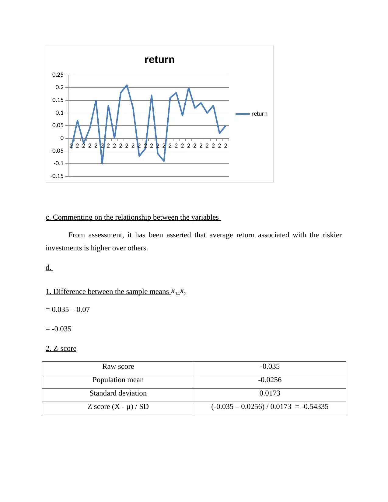
When risk level is high

2 2 2 2 2 2 2 2 2 2 2 2 2 2 2 2 2 2 2 2 2 2 2 2 2 2
-0.15
-0.1
-0.05
0
0.05
0.1
0.15
0.2
0.25
return
return
c. Commenting on the relationship between the variables
From assessment, it has been asserted that average return associated with the riskier
investments is higher over others.
d.
1. Difference between the sample means x1-x2
= 0.035 – 0.07
= -0.035
2. Z-score
Raw score -0.035
Population mean -0.0256
Standard deviation 0.0173
Z score (X - μ) / SD (-0.035 – 0.0256) / 0.0173 = -0.54335

3.
4.
Expected rank = P(Z<zscore)*2000
= .293 * 2000
= 586

e. Testing significant differences in the mean value @ 5% level of significance
1. Hypothesis
H0: There is no significant difference takes place in the returns offered by different kind of
investments.
H1: There is a significant difference takes place in the returns offered by different kind of
investments.
2.
Results
Difference 0.035
Standard error 0.020
95% CI -0.0037 to 0.0737
t-statistic 1.794
DF 98
Significance level P = 0.0759
3.
H0: Rejected (P>0.0759)
4.
By considering the results of statistical analysis, it can be depicted that mean returns
offered by both kind of investment do not vary to a great extent.

SECTION 4
a.
Row Labels Count of do you support proposed change?
no 88
yes 112
Grand Total 200
b.
Sample size: 200 people
Sample proportion:
Particulars % of people
No 44%
Yes 56%
c. Assessing Z score
1.
Raw score .56
Population mean 0.6
Standard deviation .0357
Z score (X - μ) / SD (.56 – 0.6) / .0357 = -1.12
2.

3. Ranking
P (Z < zscore)*1000
= .131 * 1000
= 131
d. Finding 95% confidence interval level for the people who support change
Sample mean .6
Sample size or people who support change 112
S.D. .0357
Confidence level 95%
M 0.6, 95% CI [0.593, 0.607]

SECTION 5
A and c Creating or obtaining own data set
Work-life balance
 1 = Yes
 2 = No
Number
of
responden
ts
Gend
er
Work-life
balance
1 M 1
2 F 2
3 F 2
4 M 1
5 M 1
6 M 2
7 F 1
8 M 2
9 F 2
10 M 1
11 M 1
12 F 1
13 M 1
14 F 2
15 M 1
16 F 1
17 F 2
18 M 1
19 M 1
20 F 1
b. Summarizing variables by using pivot table
Categorical variable: Gender
Row Labels Count of Gender
F 9

M 11
Grand Total 20
Other variable: Work-life balance
Row Labels Count of Work-life balance
2 7
1 13
Grand Total 20
Interpretation: By doing assessment it has found that out of 20 respondents, 9 were
female and remaining recognized as male. In addition to this, it has been assessed that out of 20,
13 people said that they effectually managed balance between the personal and professional life
over others.
SECTION 6
Discussing the manner in which mean and standard deviations are used in finance
Mean and standard deviations are the most effectual statistical measures which in turn
help in evaluating the large data set. By dividing sum from the total numbers mean value can be
assessed. It implies for the average value of data and thereby helps in evaluating the large set.
Further, standard deviation entails the extent to which mean will change due to the fluctuations
take place in other variables. Hence, by using the outcome of both statistical measures analyst
can take appropriate decisions for near future.