STAT6003: Analysis of Financial Data Using Statistical Methods Report
VerifiedAdded on 2022/09/15
|16
|2640
|21
Report
AI Summary
This report presents a statistical analysis of financial data, focusing on regression analysis to determine the relationship between market price and various independent variables such as Sydney price index, annual percentage change, total number of square meters, and age of the house. The study employs the ordinary least squares method to build a model, including scatter plots to visualize relationships between variables and the least squares regression equation. The report evaluates the estimated coefficients, significance levels, coefficient of determination, and confidence intervals. Hypothesis testing is conducted to examine the relationship between market price and land size, followed by a goodness-of-fit assessment comparing the original and re-estimated models. Finally, the report predicts the market price of a house based on building area, providing a comprehensive statistical overview for financial decision-making, and referencing relevant literature.
Running Head: STATISTICS FOR FINANCIAL DECISIONS
Statistics for Financial Decisions
Name of the Student:
Name of the University:
Author Note:
Statistics for Financial Decisions
Name of the Student:
Name of the University:
Author Note:
Paraphrase This Document
Need a fresh take? Get an instant paraphrase of this document with our AI Paraphraser
1Running Head: STATISTICS FOR FINANCIAL DECISIONS
Table of Contents
Introduction................................................................................................................................2
Discussion..................................................................................................................................3
Scatter plot on market price versus annual % change............................................................4
Scatter plot on total number of square meters versus Sydney price......................................5
Scatter plot on age of house versus Sydney price..................................................................6
Assignment model..................................................................................................................7
Least square regression..........................................................................................................7
Estimated and significant value of the model........................................................................7
Coefficient of determination..................................................................................................8
Confidence interval................................................................................................................9
Hypothesis test.....................................................................................................................10
Goodness of fit.....................................................................................................................10
Prediction of Dependent variable.........................................................................................11
Conclusion................................................................................................................................12
References................................................................................................................................13
2Running Head: STATISTICS FOR FINANCIAL DECISIONS
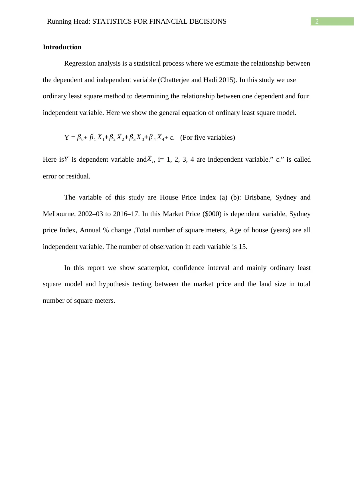
Introduction
Regression analysis is a statistical process where we estimate the relationship between
the dependent and independent variable (Chatterjee and Hadi 2015). In this study we use
ordinary least square method to determining the relationship between one dependent and four
independent variable. Here we show the general equation of ordinary least square model.
Y = β0+ β1 X1+ β2 X2 +β3 X 3+ β 4 X4+ ε. (For five variables)
Here isY is dependent variable and Xi, i= 1, 2, 3, 4 are independent variable.” ε.” is called
error or residual.
The variable of this study are House Price Index (a) (b): Brisbane, Sydney and
Melbourne, 2002–03 to 2016–17. In this Market Price ($000) is dependent variable, Sydney
price Index, Annual % change ,Total number of square meters, Age of house (years) are all
independent variable. The number of observation in each variable is 15.
In this report we show scatterplot, confidence interval and mainly ordinary least
square model and hypothesis testing between the market price and the land size in total
number of square meters.
⊘ This is a preview!⊘
Do you want full access?
Subscribe today to unlock all pages.
Trusted by 1+ million students worldwide
3Running Head: STATISTICS FOR FINANCIAL DECISIONS
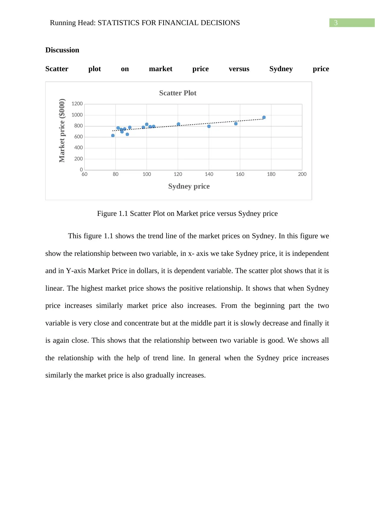
Discussion
Scatter plot on market price versus Sydney price
60 80 100 120 140 160 180 200
0
200
400
600
800
1000
1200
Scatter Plot
Sydney price
Market price ($000)
Figure 1.1 Scatter Plot on Market price versus Sydney price
This figure 1.1 shows the trend line of the market prices on Sydney. In this figure we
show the relationship between two variable, in x- axis we take Sydney price, it is independent
and in Y-axis Market Price in dollars, it is dependent variable. The scatter plot shows that it is
linear. The highest market price shows the positive relationship. It shows that when Sydney
price increases similarly market price also increases. From the beginning part the two
variable is very close and concentrate but at the middle part it is slowly decrease and finally it
is again close. This shows that the relationship between two variable is good. We shows all
the relationship with the help of trend line. In general when the Sydney price increases
similarly the market price is also gradually increases.
Paraphrase This Document
Need a fresh take? Get an instant paraphrase of this document with our AI Paraphraser
4Running Head: STATISTICS FOR FINANCIAL DECISIONS
Scatter plot on market price versus annual % change
0 2 4 6 8 10 12 14 16 18
0
200
400
600
800
1000
1200
Scatter Plot
Annual % change
Market Price($000)
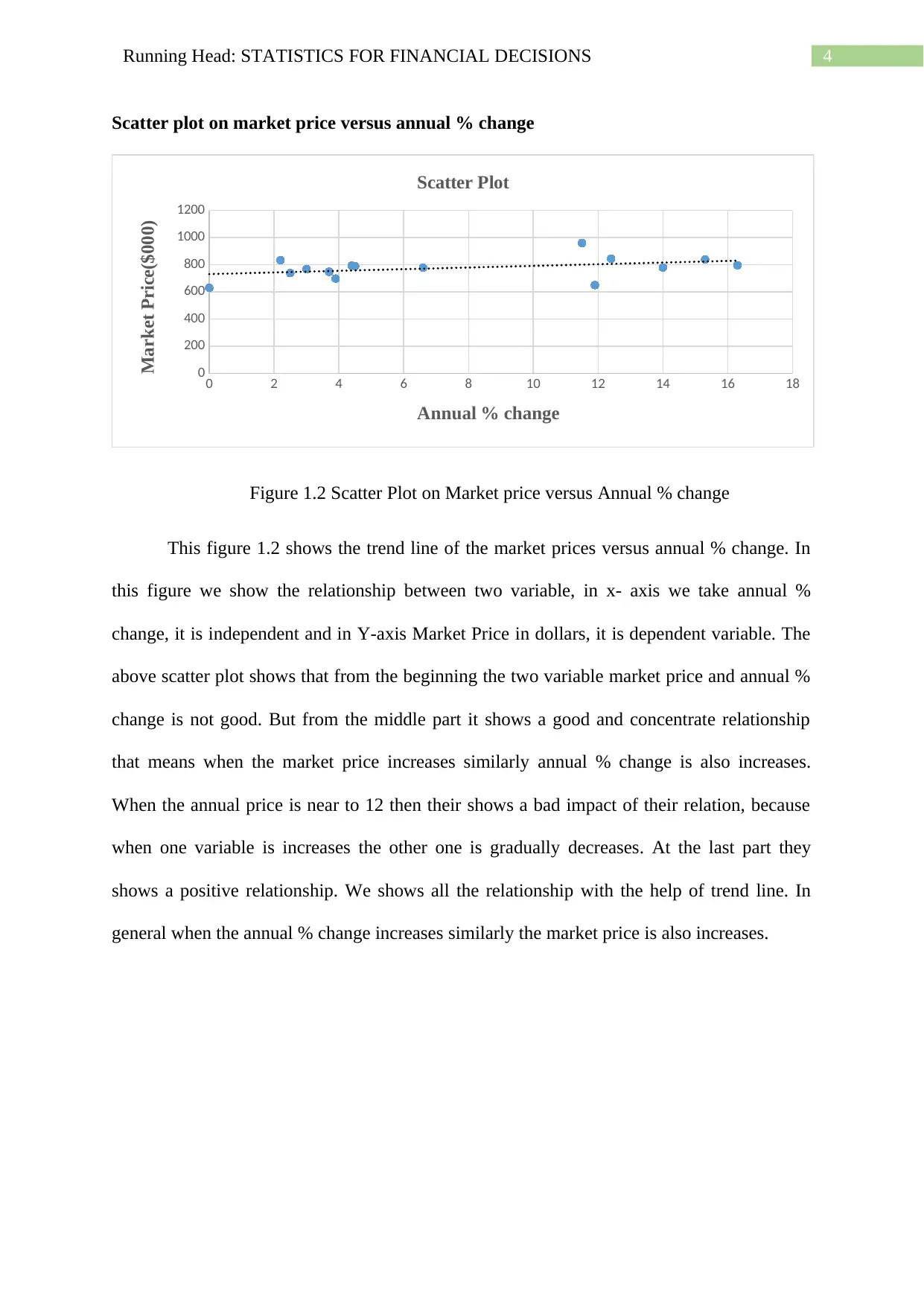
Figure 1.2 Scatter Plot on Market price versus Annual % change
This figure 1.2 shows the trend line of the market prices versus annual % change. In
this figure we show the relationship between two variable, in x- axis we take annual %
change, it is independent and in Y-axis Market Price in dollars, it is dependent variable. The
above scatter plot shows that from the beginning the two variable market price and annual %
change is not good. But from the middle part it shows a good and concentrate relationship
that means when the market price increases similarly annual % change is also increases.
When the annual price is near to 12 then their shows a bad impact of their relation, because
when one variable is increases the other one is gradually decreases. At the last part they
shows a positive relationship. We shows all the relationship with the help of trend line. In
general when the annual % change increases similarly the market price is also increases.
Scatter plot on market price versus annual % change
0 2 4 6 8 10 12 14 16 18
0
200
400
600
800
1000
1200
Scatter Plot
Annual % change
Market Price($000)
Figure 1.2 Scatter Plot on Market price versus Annual % change
This figure 1.2 shows the trend line of the market prices versus annual % change. In
this figure we show the relationship between two variable, in x- axis we take annual %
change, it is independent and in Y-axis Market Price in dollars, it is dependent variable. The
above scatter plot shows that from the beginning the two variable market price and annual %
change is not good. But from the middle part it shows a good and concentrate relationship
that means when the market price increases similarly annual % change is also increases.
When the annual price is near to 12 then their shows a bad impact of their relation, because
when one variable is increases the other one is gradually decreases. At the last part they
shows a positive relationship. We shows all the relationship with the help of trend line. In
general when the annual % change increases similarly the market price is also increases.
5Running Head: STATISTICS FOR FINANCIAL DECISIONS
Scatter plot on total number of square meters versus Sydney price
140 160 180 200 220 240 260 280 300 320
0
200
400
600
800
1000
1200
Scatter Plot
Total number of square meters
Market Price ($000)
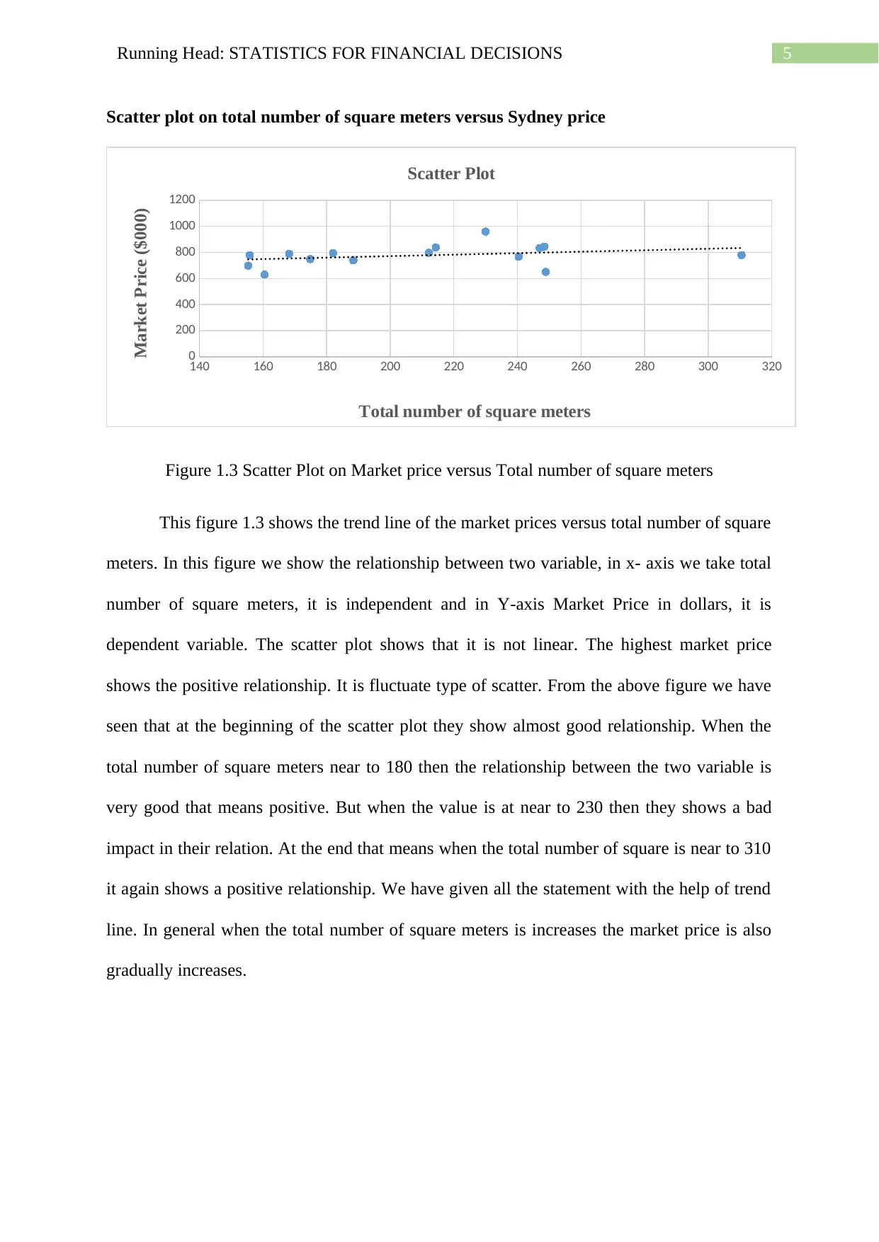
Figure 1.3 Scatter Plot on Market price versus Total number of square meters
This figure 1.3 shows the trend line of the market prices versus total number of square
meters. In this figure we show the relationship between two variable, in x- axis we take total
number of square meters, it is independent and in Y-axis Market Price in dollars, it is
dependent variable. The scatter plot shows that it is not linear. The highest market price
shows the positive relationship. It is fluctuate type of scatter. From the above figure we have
seen that at the beginning of the scatter plot they show almost good relationship. When the
total number of square meters near to 180 then the relationship between the two variable is
very good that means positive. But when the value is at near to 230 then they shows a bad
impact in their relation. At the end that means when the total number of square is near to 310
it again shows a positive relationship. We have given all the statement with the help of trend
line. In general when the total number of square meters is increases the market price is also
gradually increases.
Scatter plot on total number of square meters versus Sydney price
140 160 180 200 220 240 260 280 300 320
0
200
400
600
800
1000
1200
Scatter Plot
Total number of square meters
Market Price ($000)
Figure 1.3 Scatter Plot on Market price versus Total number of square meters
This figure 1.3 shows the trend line of the market prices versus total number of square
meters. In this figure we show the relationship between two variable, in x- axis we take total
number of square meters, it is independent and in Y-axis Market Price in dollars, it is
dependent variable. The scatter plot shows that it is not linear. The highest market price
shows the positive relationship. It is fluctuate type of scatter. From the above figure we have
seen that at the beginning of the scatter plot they show almost good relationship. When the
total number of square meters near to 180 then the relationship between the two variable is
very good that means positive. But when the value is at near to 230 then they shows a bad
impact in their relation. At the end that means when the total number of square is near to 310
it again shows a positive relationship. We have given all the statement with the help of trend
line. In general when the total number of square meters is increases the market price is also
gradually increases.
⊘ This is a preview!⊘
Do you want full access?
Subscribe today to unlock all pages.
Trusted by 1+ million students worldwide
6Running Head: STATISTICS FOR FINANCIAL DECISIONS
Scatter plot on age of house versus Sydney price
0 5 10 15 20 25 30 35 40 45 50
0
200
400
600
800
1000
1200
Scatter Plot
Age of house (years)
Market Price ($000)
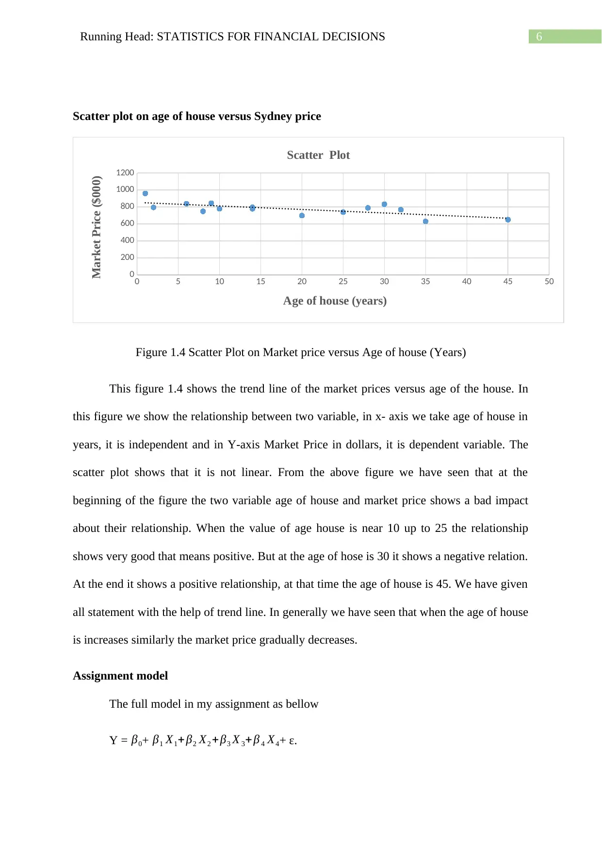
Figure 1.4 Scatter Plot on Market price versus Age of house (Years)
This figure 1.4 shows the trend line of the market prices versus age of the house. In
this figure we show the relationship between two variable, in x- axis we take age of house in
years, it is independent and in Y-axis Market Price in dollars, it is dependent variable. The
scatter plot shows that it is not linear. From the above figure we have seen that at the
beginning of the figure the two variable age of house and market price shows a bad impact
about their relationship. When the value of age house is near 10 up to 25 the relationship
shows very good that means positive. But at the age of hose is 30 it shows a negative relation.
At the end it shows a positive relationship, at that time the age of house is 45. We have given
all statement with the help of trend line. In generally we have seen that when the age of house
is increases similarly the market price gradually decreases.
Assignment model
The full model in my assignment as bellow
Y = β0+ β1 X1+ β2 X2 +β3 X 3+ β 4 X4+ ε.
Scatter plot on age of house versus Sydney price
0 5 10 15 20 25 30 35 40 45 50
0
200
400
600
800
1000
1200
Scatter Plot
Age of house (years)
Market Price ($000)
Figure 1.4 Scatter Plot on Market price versus Age of house (Years)
This figure 1.4 shows the trend line of the market prices versus age of the house. In
this figure we show the relationship between two variable, in x- axis we take age of house in
years, it is independent and in Y-axis Market Price in dollars, it is dependent variable. The
scatter plot shows that it is not linear. From the above figure we have seen that at the
beginning of the figure the two variable age of house and market price shows a bad impact
about their relationship. When the value of age house is near 10 up to 25 the relationship
shows very good that means positive. But at the age of hose is 30 it shows a negative relation.
At the end it shows a positive relationship, at that time the age of house is 45. We have given
all statement with the help of trend line. In generally we have seen that when the age of house
is increases similarly the market price gradually decreases.
Assignment model
The full model in my assignment as bellow
Y = β0+ β1 X1+ β2 X2 +β3 X 3+ β 4 X4+ ε.
Paraphrase This Document
Need a fresh take? Get an instant paraphrase of this document with our AI Paraphraser
7Running Head: STATISTICS FOR FINANCIAL DECISIONS
Here isY is dependent variable andXi, i= 1, 2, 3, 4 are independent variable.” ε.” is called
error or residual.
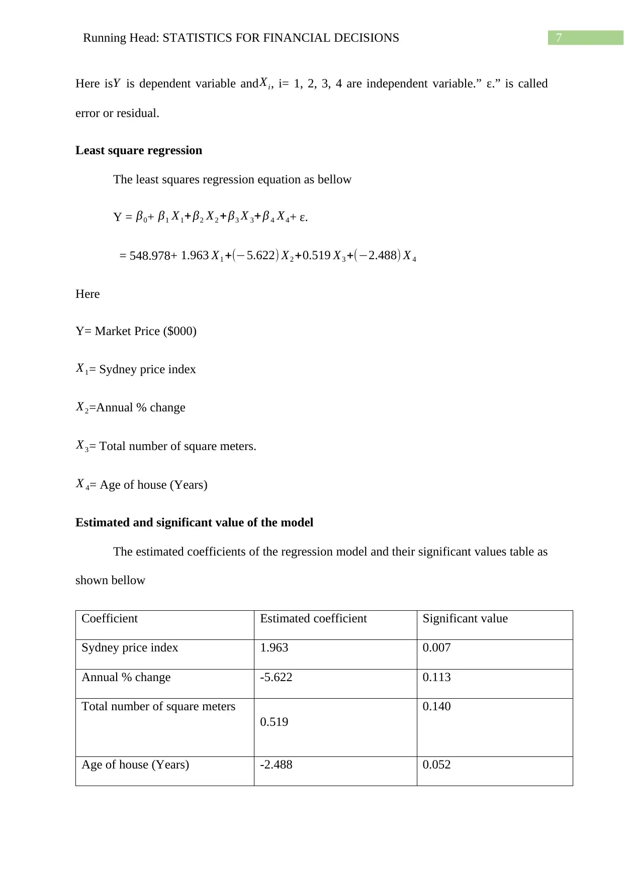
Least square regression
The least squares regression equation as bellow
Y = β0+ β1 X1+ β2 X2 +β3 X 3+ β 4 X4+ ε.
= 548.978+ 1.963 X1 +(−5.622) X2 +0.519 X3 +(−2.488) X 4
Here
Y= Market Price ($000)
X1= Sydney price index
X2=Annual % change
X3= Total number of square meters.
X 4= Age of house (Years)
Estimated and significant value of the model
The estimated coefficients of the regression model and their significant values table as
shown bellow
Coefficient Estimated coefficient Significant value
Sydney price index 1.963 0.007
Annual % change -5.622 0.113
Total number of square meters
0.519
0.140
Age of house (Years) -2.488 0.052
Here isY is dependent variable andXi, i= 1, 2, 3, 4 are independent variable.” ε.” is called
error or residual.
Least square regression
The least squares regression equation as bellow
Y = β0+ β1 X1+ β2 X2 +β3 X 3+ β 4 X4+ ε.
= 548.978+ 1.963 X1 +(−5.622) X2 +0.519 X3 +(−2.488) X 4
Here
Y= Market Price ($000)
X1= Sydney price index
X2=Annual % change
X3= Total number of square meters.
X 4= Age of house (Years)
Estimated and significant value of the model
The estimated coefficients of the regression model and their significant values table as
shown bellow
Coefficient Estimated coefficient Significant value
Sydney price index 1.963 0.007
Annual % change -5.622 0.113
Total number of square meters
0.519
0.140
Age of house (Years) -2.488 0.052

8Running Head: STATISTICS FOR FINANCIAL DECISIONS
Table 1.1 Estimated coefficient and significant value
From the above table we have seen that for Sydney price index the estimated value is
larger than the significant value. It is good, because if we see at 5% level of significance than
it gives a good result.
In case of annual % change the estimated value is lesser than the significant value. It
is good, because if we see at 5% level of significance than it gives a good result.
In case of Total number of square meters the estimated value is larger than the
significant value. It is good, because if we see at 5% level of significance than it gives a good
result.
Similarly, in case of Age of the house (in years) the estimated value is larger than the
significant value. It is good, because if we see at 5% level of significance than it gives a good
result.
Coefficient of determination
The coefficient of determination for the relationship between the dependent and
independent variables is 0.7906 that is 79%.
Here the R-square value is 0.7906 and R-square adjusted is 0.7069.
Since R-square > R-square adjusted. That is in the model independent of attributes is
correlated.
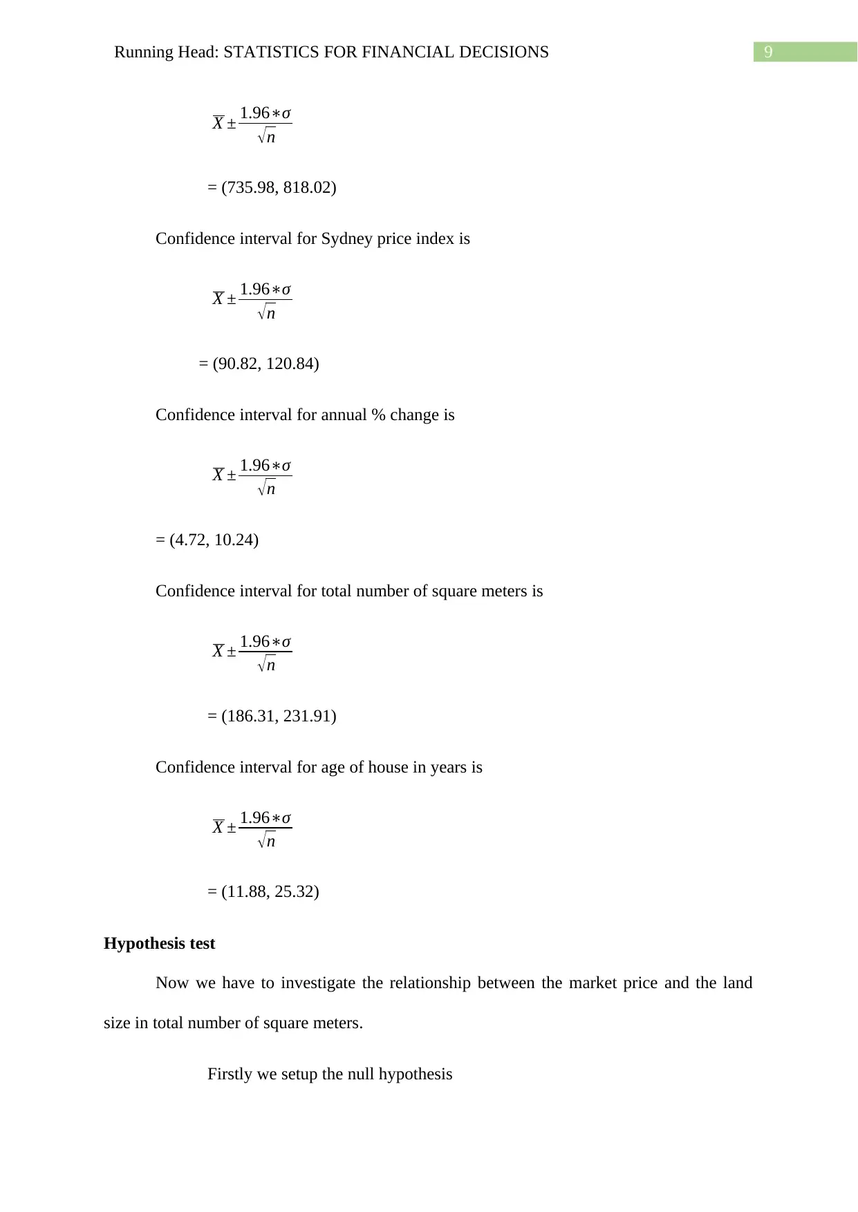
Confidence interval
The 95% confidence intervals for each parameters and interpret these intervals as
bellow
Confidence interval for market price is
Table 1.1 Estimated coefficient and significant value
From the above table we have seen that for Sydney price index the estimated value is
larger than the significant value. It is good, because if we see at 5% level of significance than
it gives a good result.
In case of annual % change the estimated value is lesser than the significant value. It
is good, because if we see at 5% level of significance than it gives a good result.
In case of Total number of square meters the estimated value is larger than the
significant value. It is good, because if we see at 5% level of significance than it gives a good
result.
Similarly, in case of Age of the house (in years) the estimated value is larger than the
significant value. It is good, because if we see at 5% level of significance than it gives a good
result.
Coefficient of determination
The coefficient of determination for the relationship between the dependent and
independent variables is 0.7906 that is 79%.
Here the R-square value is 0.7906 and R-square adjusted is 0.7069.
Since R-square > R-square adjusted. That is in the model independent of attributes is
correlated.
Confidence interval
The 95% confidence intervals for each parameters and interpret these intervals as
bellow
Confidence interval for market price is
⊘ This is a preview!⊘
Do you want full access?
Subscribe today to unlock all pages.
Trusted by 1+ million students worldwide
9Running Head: STATISTICS FOR FINANCIAL DECISIONS
X ± 1.96∗σ
√n
= (735.98, 818.02)
Confidence interval for Sydney price index is
X ± 1.96∗σ
√n
= (90.82, 120.84)
Confidence interval for annual % change is
X ± 1.96∗σ
√n
= (4.72, 10.24)
Confidence interval for total number of square meters is
X ± 1.96∗σ
√n
= (186.31, 231.91)
Confidence interval for age of house in years is
X ± 1.96∗σ
√n
= (11.88, 25.32)
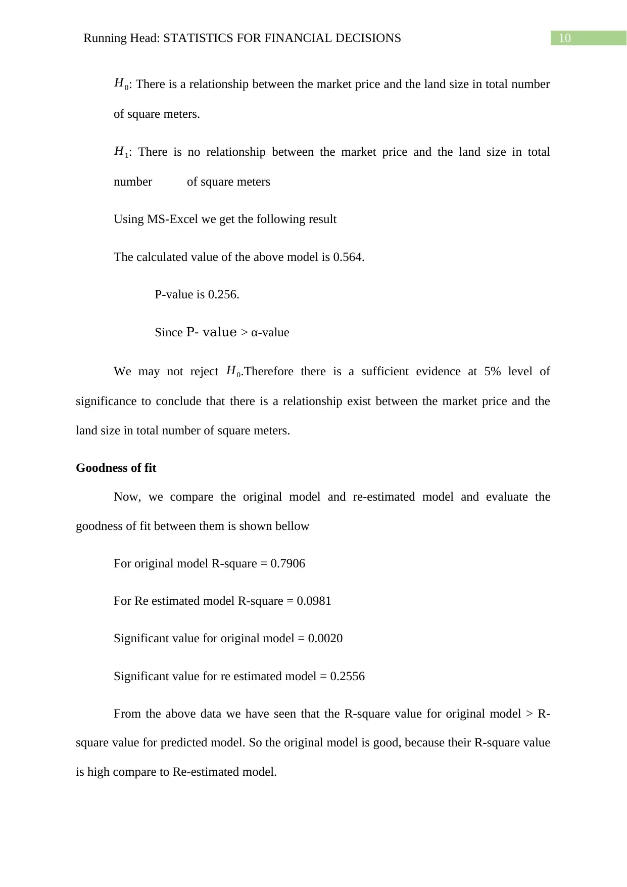
Hypothesis test
Now we have to investigate the relationship between the market price and the land
size in total number of square meters.
Firstly we setup the null hypothesis
X ± 1.96∗σ
√n
= (735.98, 818.02)
Confidence interval for Sydney price index is
X ± 1.96∗σ
√n
= (90.82, 120.84)
Confidence interval for annual % change is
X ± 1.96∗σ
√n
= (4.72, 10.24)
Confidence interval for total number of square meters is
X ± 1.96∗σ
√n
= (186.31, 231.91)
Confidence interval for age of house in years is
X ± 1.96∗σ
√n
= (11.88, 25.32)
Hypothesis test
Now we have to investigate the relationship between the market price and the land
size in total number of square meters.
Firstly we setup the null hypothesis
Paraphrase This Document
Need a fresh take? Get an instant paraphrase of this document with our AI Paraphraser
10Running Head: STATISTICS FOR FINANCIAL DECISIONS
H0: There is a relationship between the market price and the land size in total number
of square meters.
H1: There is no relationship between the market price and the land size in total
number of square meters
Using MS-Excel we get the following result
The calculated value of the above model is 0.564.
P-value is 0.256.
Since P- value > α-value
We may not reject H0.Therefore there is a sufficient evidence at 5% level of
significance to conclude that there is a relationship exist between the market price and the
land size in total number of square meters.
Goodness of fit
Now, we compare the original model and re-estimated model and evaluate the
goodness of fit between them is shown bellow
For original model R-square = 0.7906
For Re estimated model R-square = 0.0981
Significant value for original model = 0.0020
Significant value for re estimated model = 0.2556
From the above data we have seen that the R-square value for original model > R-
square value for predicted model. So the original model is good, because their R-square value
is high compare to Re-estimated model.
11Running Head: STATISTICS FOR FINANCIAL DECISIONS
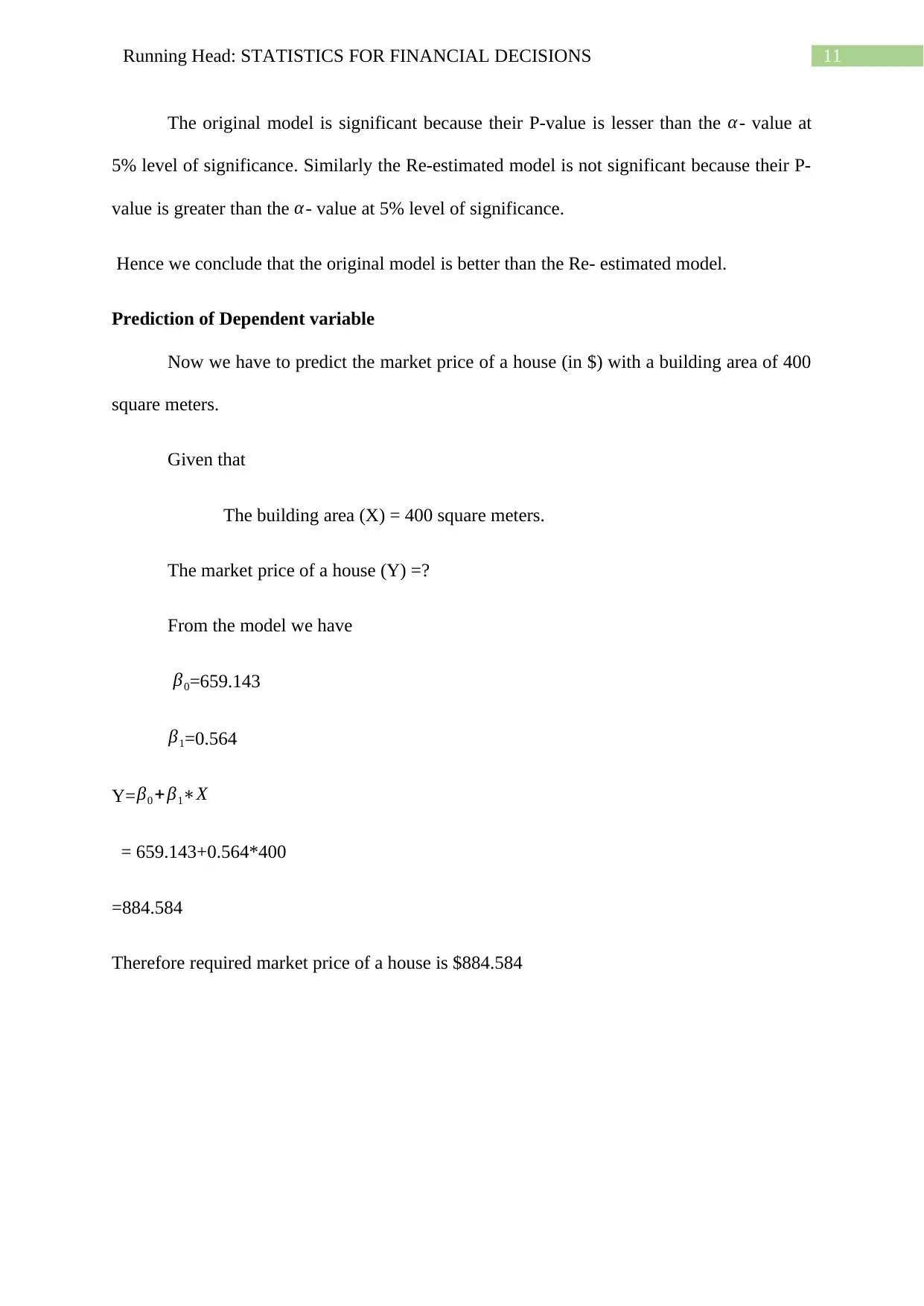
The original model is significant because their P-value is lesser than the α- value at
5% level of significance. Similarly the Re-estimated model is not significant because their P-
value is greater than the α- value at 5% level of significance.
Hence we conclude that the original model is better than the Re- estimated model.
Prediction of Dependent variable
Now we have to predict the market price of a house (in $) with a building area of 400
square meters.
Given that
The building area (X) = 400 square meters.
The market price of a house (Y) =?
From the model we have
β0=659.143
β1=0.564
Y=β0 +β1∗X
= 659.143+0.564*400
=884.584
Therefore required market price of a house is $884.584
⊘ This is a preview!⊘
Do you want full access?
Subscribe today to unlock all pages.
Trusted by 1+ million students worldwide
1 out of 16
Related Documents


Your All-in-One AI-Powered Toolkit for Academic Success.
+13062052269
info@desklib.com
Available 24*7 on WhatsApp / Email
![[object Object]](/_next/static/media/star-bottom.7253800d.svg)
Unlock your academic potential
Copyright © 2020–2026 A2Z Services. All Rights Reserved. Developed and managed by ZUCOL.