Statistics for Financial Decisions | Assignment
VerifiedAdded on 2022/09/18
|11
|1840
|19
AI Summary
Contribute Materials
Your contribution can guide someone’s learning journey. Share your
documents today.
Running head: STATISTICS FOR FINANCIAL DECISIONS
Statistics for Financial Decisions
Name of the University:
Name of the student:
Authors Note:
Statistics for Financial Decisions
Name of the University:
Name of the student:
Authors Note:
Secure Best Marks with AI Grader
Need help grading? Try our AI Grader for instant feedback on your assignments.
1STATISTICS FOR FINANCIAL DECISIONS
Table of Contents
a) Introduction:...........................................................................................................................2
b) Relationship between dependent and independent variables using scatterplots....................2
Fig 1. Scatter Plot between age of house and market price...................................................2
Fig 2. Scatter plot between price index and the market price................................................3
Fig 3. Scatter plot between Area and Market Price...............................................................3
c) Multiple Regression Summary Statistics:..............................................................................4
e) Slope of simple linear regression:..........................................................................................5
f) Co-efficient of determination for simple linear regression:...................................................6
g) 95% confidence interval for the slope coefficient................................................................6
h) Goodness of fit.......................................................................................................................6
i) Predicting Market Price..........................................................................................................6
j) Hypothesis Test......................................................................................................................7
References:.................................................................................................................................9
2STATISTICS FOR FINANCIAL DECISIONS
a) Introduction:
The data of 400 variables all related to the real estate sector is given. The variables are
Property Id, Market Price of house in dollars, Property Index, Size of house in square metres
and Age of the house in years. Generally, in the real estate industry, the price of a house of
increases with increase in size of the house. And the more the age of the house the lesser its
price due to depreciation. The price of a house is dependent on many other factors such as the
neighbourhood, the number of bedrooms, the price index, local taxes etc(Ihlanfeldt, 2007). In
this report, the data is calculated for four parameters. Out of the 400 data entries, 50 random
samples are selected with the aid of a random number table.
The OLS regression is used for estimating if there is any relationship between, the market
price of a house and the other variables. The market price is taken as the response variable
and the price index, size of the house and age of the house are taken as the explanatory
variables (Chatterjee and Hadi,2015).
b) Relationship between dependent and independent variables using scatterplots.
-5 0 5 10 15 20 25 30 35 40 45
0
100
200
300
400
500
600
700
800
900
1000
f(x) = 0.174616926132148 x + 758.053443743358
R² = 0.00086003369532528
Scatter Plot
Age
Market Price.
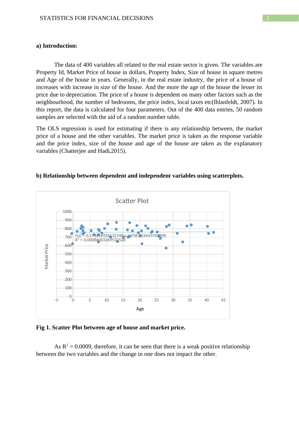
Fig 1. Scatter Plot between age of house and market price.
As R2 = 0.0009, therefore, it can be seen that there is a weak positive relationship
between the two variables and the change in one does not impact the other.
a) Introduction:
The data of 400 variables all related to the real estate sector is given. The variables are
Property Id, Market Price of house in dollars, Property Index, Size of house in square metres
and Age of the house in years. Generally, in the real estate industry, the price of a house of
increases with increase in size of the house. And the more the age of the house the lesser its
price due to depreciation. The price of a house is dependent on many other factors such as the
neighbourhood, the number of bedrooms, the price index, local taxes etc(Ihlanfeldt, 2007). In
this report, the data is calculated for four parameters. Out of the 400 data entries, 50 random
samples are selected with the aid of a random number table.
The OLS regression is used for estimating if there is any relationship between, the market
price of a house and the other variables. The market price is taken as the response variable
and the price index, size of the house and age of the house are taken as the explanatory
variables (Chatterjee and Hadi,2015).
b) Relationship between dependent and independent variables using scatterplots.
-5 0 5 10 15 20 25 30 35 40 45
0
100
200
300
400
500
600
700
800
900
1000
f(x) = 0.174616926132148 x + 758.053443743358
R² = 0.00086003369532528
Scatter Plot
Age
Market Price.
Fig 1. Scatter Plot between age of house and market price.
As R2 = 0.0009, therefore, it can be seen that there is a weak positive relationship
between the two variables and the change in one does not impact the other.
3STATISTICS FOR FINANCIAL DECISIONS
20.0 40.0 60.0 80.0 100.0 120.0 140.0 160.0 180.0
0
100
200
300
400
500
600
700
800
900
1000
f(x) = 0.160569912482998 x + 743.741891359312R² = 0.00380086559761694
Scatter Plot
Price Index
Market Price
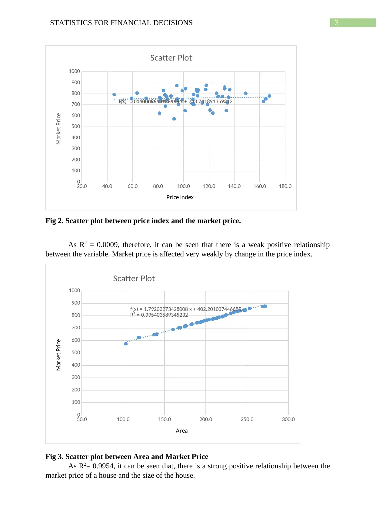
Fig 2. Scatter plot between price index and the market price.
As R2 = 0.0009, therefore, it can be seen that there is a weak positive relationship
between the variable. Market price is affected very weakly by change in the price index.
50.0 100.0 150.0 200.0 250.0 300.0
0
100
200
300
400
500
600
700
800
900
1000
f(x) = 1.79202273428008 x + 402.201037446685
R² = 0.995403589345232
Scatter Plot
Area
Market Price
Fig 3. Scatter plot between Area and Market Price
As R2= 0.9954, it can be seen that, there is a strong positive relationship between the
market price of a house and the size of the house.
20.0 40.0 60.0 80.0 100.0 120.0 140.0 160.0 180.0
0
100
200
300
400
500
600
700
800
900
1000
f(x) = 0.160569912482998 x + 743.741891359312R² = 0.00380086559761694
Scatter Plot
Price Index
Market Price
Fig 2. Scatter plot between price index and the market price.
As R2 = 0.0009, therefore, it can be seen that there is a weak positive relationship
between the variable. Market price is affected very weakly by change in the price index.
50.0 100.0 150.0 200.0 250.0 300.0
0
100
200
300
400
500
600
700
800
900
1000
f(x) = 1.79202273428008 x + 402.201037446685
R² = 0.995403589345232
Scatter Plot
Area
Market Price
Fig 3. Scatter plot between Area and Market Price
As R2= 0.9954, it can be seen that, there is a strong positive relationship between the
market price of a house and the size of the house.
Secure Best Marks with AI Grader
Need help grading? Try our AI Grader for instant feedback on your assignments.
4STATISTICS FOR FINANCIAL DECISIONS
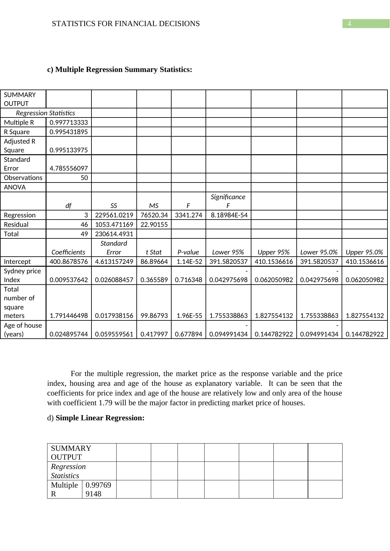
c) Multiple Regression Summary Statistics:
SUMMARY
OUTPUT
Regression Statistics
Multiple R 0.997713333
R Square 0.995431895
Adjusted R
Square 0.995133975
Standard
Error 4.785556097
Observations 50
ANOVA
df SS MS F
Significance
F
Regression 3 229561.0219 76520.34 3341.274 8.18984E-54
Residual 46 1053.471169 22.90155
Total 49 230614.4931
Coefficients
Standard
Error t Stat P-value Lower 95% Upper 95% Lower 95.0% Upper 95.0%
Intercept 400.8678576 4.613157249 86.89664 1.14E-52 391.5820537 410.1536616 391.5820537 410.1536616
Sydney price
Index 0.009537642 0.026088457 0.365589 0.716348
-
0.042975698 0.062050982
-
0.042975698 0.062050982
Total
number of
square
meters 1.791446498 0.017938156 99.86793 1.96E-55 1.755338863 1.827554132 1.755338863 1.827554132
Age of house
(years) 0.024895744 0.059559561 0.417997 0.677894
-
0.094991434 0.144782922
-
0.094991434 0.144782922
For the multiple regression, the market price as the response variable and the price
index, housing area and age of the house as explanatory variable. It can be seen that the
coefficients for price index and age of the house are relatively low and only area of the house
with coefficient 1.79 will be the major factor in predicting market price of houses.
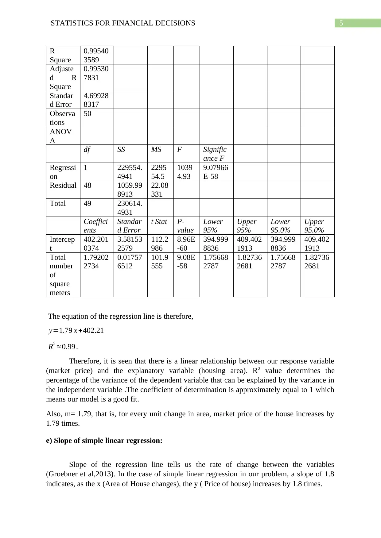
d) Simple Linear Regression:
SUMMARY
OUTPUT
Regression
Statistics
Multiple
R
0.99769
9148
c) Multiple Regression Summary Statistics:
SUMMARY
OUTPUT
Regression Statistics
Multiple R 0.997713333
R Square 0.995431895
Adjusted R
Square 0.995133975
Standard
Error 4.785556097
Observations 50
ANOVA
df SS MS F
Significance
F
Regression 3 229561.0219 76520.34 3341.274 8.18984E-54
Residual 46 1053.471169 22.90155
Total 49 230614.4931
Coefficients
Standard
Error t Stat P-value Lower 95% Upper 95% Lower 95.0% Upper 95.0%
Intercept 400.8678576 4.613157249 86.89664 1.14E-52 391.5820537 410.1536616 391.5820537 410.1536616
Sydney price
Index 0.009537642 0.026088457 0.365589 0.716348
-
0.042975698 0.062050982
-
0.042975698 0.062050982
Total
number of
square
meters 1.791446498 0.017938156 99.86793 1.96E-55 1.755338863 1.827554132 1.755338863 1.827554132
Age of house
(years) 0.024895744 0.059559561 0.417997 0.677894
-
0.094991434 0.144782922
-
0.094991434 0.144782922
For the multiple regression, the market price as the response variable and the price
index, housing area and age of the house as explanatory variable. It can be seen that the
coefficients for price index and age of the house are relatively low and only area of the house
with coefficient 1.79 will be the major factor in predicting market price of houses.
d) Simple Linear Regression:
SUMMARY
OUTPUT
Regression
Statistics
Multiple
R
0.99769
9148
5STATISTICS FOR FINANCIAL DECISIONS
R
Square
0.99540
3589
Adjuste
d R
Square
0.99530
7831
Standar
d Error
4.69928
8317
Observa
tions
50
ANOV
A
df SS MS F Signific
ance F
Regressi
on
1 229554.
4941
2295
54.5
1039
4.93
9.07966
E-58
Residual 48 1059.99
8913
22.08
331
Total 49 230614.
4931
Coeffici
ents
Standar
d Error
t Stat P-
value
Lower
95%
Upper
95%
Lower
95.0%
Upper
95.0%
Intercep
t
402.201
0374
3.58153
2579
112.2
986
8.96E
-60
394.999
8836
409.402
1913
394.999
8836
409.402
1913
Total
number
of
square
meters
1.79202
2734
0.01757
6512
101.9
555
9.08E
-58
1.75668
2787
1.82736
2681
1.75668
2787
1.82736
2681
The equation of the regression line is therefore,
y=1.79 x +402.21
R2 ≈ 0.99 .
Therefore, it is seen that there is a linear relationship between our response variable
(market price) and the explanatory variable (housing area). R2 value determines the
percentage of the variance of the dependent variable that can be explained by the variance in
the independent variable .The coefficient of determination is approximately equal to 1 which
means our model is a good fit.
Also, m= 1.79, that is, for every unit change in area, market price of the house increases by
1.79 times.
e) Slope of simple linear regression:
Slope of the regression line tells us the rate of change between the variables
(Groebner et al,2013). In the case of simple linear regression in our problem, a slope of 1.8
indicates, as the x (Area of House changes), the y ( Price of house) increases by 1.8 times.
6STATISTICS FOR FINANCIAL DECISIONS
f) Co-efficient of determination for simple linear regression:
The coefficient of determination is given by R2. In this question it is 0.99. Coefficient
of determination indicates the value that determines the percentage of the variance of the
dependent variable that can be explained by the variance in the independent variable .The
coefficient of determination is approximately equal to 1 which means our model is a good fit.
g) 95% confidence interval for the slope coefficient
We can construct a confidence interval for the population slope ( β1 ) from our sample
slope.
i.e b1 ± t¿ (SEb1
).
b1 is the sample slope,
t¿ is the test statistic from the t distribution for degrees of freedom df = n-2,
N is the sample size.
SEb1 is the standard error of b1.
Df (degree of freedom) = 50 – 2 = 48.
Here, b1=1.79, SEb1= 0.017,
From t table we have t¿= 2.021.( T distribution table, 2019).
∴ Confidenceinterval=1.8 ±2.021 ×0.017
= (1.76, 1.834).
Thus, we have 95% confidence interval that the population slope is between 1.76 and 1.834.
h) Goodness of fit
Goodness of fit of the models can be compared by taking the R squared value
(Groebner et al., 2013) i.e coefficient of determination. The higher the coefficient of
determination the better is the fit. From the regression it is seen that R2(Linear) ≈ 0.995952617
and R2(Multilinear) ≈0.995981434.
Thus both the models are almost equal in their goodness of fit.
i) Predicting Market Price
Paraphrase This Document
Need a fresh take? Get an instant paraphrase of this document with our AI Paraphraser
7STATISTICS FOR FINANCIAL DECISIONS
Market price of a house with building area of 250 square metres:
Putting x= 250 in our regression equation we have,
y=1.79 × 250+ 402.21
= 849.71
The market price at area 250 m2 is predicted to be around 849.71.
From the original excel table with the data of 400 variables, it is seen that for land size of
249.2 the market price is equivalent to 849 and for land size 250.2 market price is equivalent
to 852.
Thus estimate of market price 849.71 corresponding to land size 250 is reasonable.
j) Hypothesis Test
For hypothesis testing, let’s formulate the null hypothesis that there is no significant
relationship between land size and the market price of a house. And the significance level is
set at 0.01.
The calculated regression equation from the sample plot between land size and market price
is y=b0 +b1x where b0=402.21 and b1=1.79 .
If the null hypothesis is true, then the population parameter, b1=0.
H0 :b1=0 , Ha :b1 ≠ 0.
From regression summary for the sample it is seen that the corresponding P value → 0.
Hence, we can reject the null hypothesis and conclude that there is significant evidence of a
relationship between land size and market price of houses.
k) Hypothesis Test for the whole model:
For the whole model, the scatter plots made for the sample, between the response and
predictor variable indicates that there might be a strong relationship between the land size and
the predictor variables and the rest of the relationships are weak for us to consider( Newey
and Macfadden, 2004). (Fig 1, Fig 2 and Fig 3)
Therefore, the hypothesis test can be done to test if there is also a significant relationship
between the land size and market price of the house. The null and alternative hypothesis are
stated below.
H0 : β=0 , Ha : β ≠ 0, where β is the slope of the model , y=β0 + β1 x .
For the sample, the regression equation for land size and market price, is
y=1.79 x +402.21 .

8STATISTICS FOR FINANCIAL DECISIONS
β=1.79∧the sample ¿ 50.
From the regression we have the t value and the corresponding p value.
T= 107.54 and p→ 0.
But the given significance level is α =0.05 which is much higher than our p value.
Therefore, we can reject our null hypothesis and accept the alternative hypothesis that there is
a significant relationship between land size and market price of a house.

9STATISTICS FOR FINANCIAL DECISIONS
Secure Best Marks with AI Grader
Need help grading? Try our AI Grader for instant feedback on your assignments.

10STATISTICS FOR FINANCIAL DECISIONS
References:
Chatterjee, S., & Hadi, A. S. (2015). Regression analysis by example. John Wiley & Sons.
Goodman, A. C. (2008). Hedonic prices, price indices and housing markets. Journal of urban
economics, 5(4), 471-484.
Green, R., & Hendershott, P. H. (2006). Age, housing demand, and real house prices.
Regional Science and Urban Economics, 26(5), 465-480.
Groebner, D. F., Shannon, P. W., Fry, P. C., & Smith, K. D. (2013). Business statistics.
Pearson Education UK.
Ihlanfeldt, K. R. (2007). The effect of land use regulation on housing and land prices.
Journal of Urban Economics, 61(3), 420-435.
Newey, W. K., & McFadden, D. (2004). Large sample estimation and hypothesis testing.
Handbook of econometrics, 4, 2111-2245.
T-Distribution Table (One Tail and Two-Tails) - Statistics How To. (2019). Statistics How
To. Retrieved 26 August 2019
Triola, M. F. (2006). Elementary statistics. Reading, MA: Pearson/Addison-Wesley.
1 out of 11
Related Documents


Your All-in-One AI-Powered Toolkit for Academic Success.
+13062052269
info@desklib.com
Available 24*7 on WhatsApp / Email
![[object Object]](/_next/static/media/star-bottom.7253800d.svg)
Unlock your academic potential
© 2024 | Zucol Services PVT LTD | All rights reserved.