Regression Analysis of House Prices

This assignment focuses on performing a regression analysis to understand the factors affecting house prices. It involves building and interpreting linear regression models, examining the significance of coefficients for variables like house size, proximity to the CBD, fireplace presence, swimming pool, and age. Students will analyze model fit using R-squared, ANOVA tables, and hypothesis testing to determine the statistically significant impact of these variables on selling price.

STATISTICS
MAE 256 T2 2017 ASSIGNMENT
STUDENT ID
[Pick the date]

Question 1
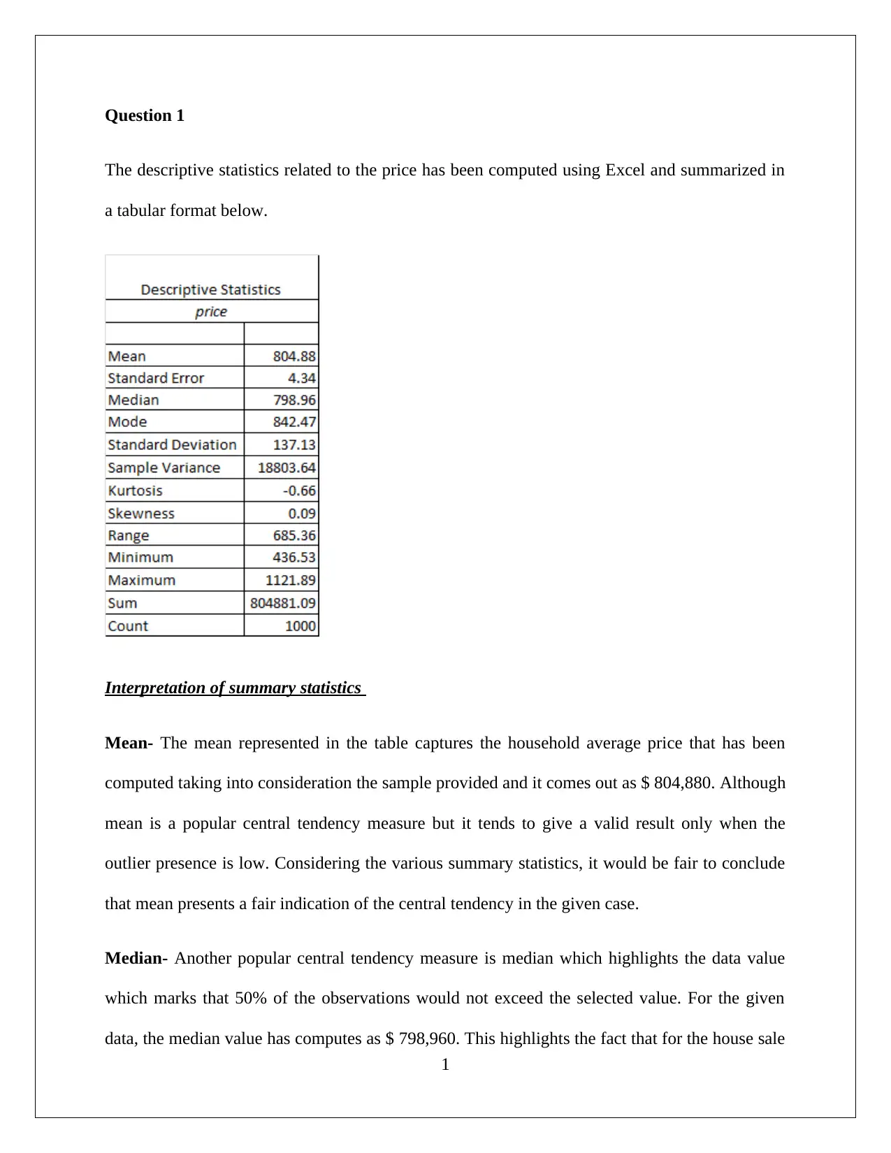
The descriptive statistics related to the price has been computed using Excel and summarized in
a tabular format below.
Interpretation of summary statistics
Mean- The mean represented in the table captures the household average price that has been
computed taking into consideration the sample provided and it comes out as $ 804,880. Although
mean is a popular central tendency measure but it tends to give a valid result only when the
outlier presence is low. Considering the various summary statistics, it would be fair to conclude
that mean presents a fair indication of the central tendency in the given case.
Median- Another popular central tendency measure is median which highlights the data value
which marks that 50% of the observations would not exceed the selected value. For the given
data, the median value has computes as $ 798,960. This highlights the fact that for the house sale
1

price presented, 50% of these have sold lower than the median value of $ 798,960. When the
skew in the distribution is minimal, there is convergence of the median and mean value which
seems to be illustrated to some extent in the given case.
Standard deviation – One of pivotal measures to capture variation is the standard deviation
which is an absolute measure. It is essential that standard deviation must be interpreted along
with the mean value so as to lead to a valid conclusion with regards to dispersion. For the selling
price of houses whose data is available, standard deviation has come out as $137,130 and when
viewed along with the mean, it is apparent that dispersion in the selling price of house seems on
the lower side. This conclusion also tends to be derived on the basis of other indicators of
dispersion in the data.
Skewness- A crucial indicator with regards to the distribution shape is the skew observed in the
data. For a normal distribution this skew ought to be zero. Further, the presence of skew implies
that a tail would be present whose respective side is driven by the sign of the skew coefficient. In
the given case, skew value is 0.09 and hence only a small tail on the right would be visible.
Question 2
The value of mean for the sale prices of houses ($ 000’s) x=804.88
The value of standard deviation for the sale prices of houses ($ 000’s) s=137.13
Proportion of houses with the sale prices within 1-standard deviation from the mean value =?
The upper and lower range of 1-standard deviation from the mean value would be computed as
given below:
2

 Upper range of 1-standard deviation from the mean value ¿ x + ( 1∗s )
¿ 804.88+ ( 1∗( 137.13 ) )
¿ 942.007
 Lower range of 1-standard deviation from the mean value ¿ x− ( 1∗s )
¿ 804.88−¿
¿ 667.75
Requisite range: (667.75 942.007)
Further, the total number of houses that lie within the above highlighted price range
¿ 638(¿ excel)
Sample size (Number of houses) ¿ 1000
Hence,
The proportion would be determined as given below:
Proportion=( 638
1000 )=0.638
Therefore, it can be said that nearly “0.638 proportion of the houses lie within the sale price of 1-
standard deviation from the mean value of houses.”
3

Question 3
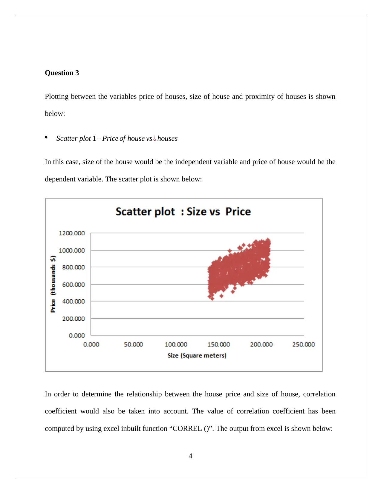
Plotting between the variables price of houses, size of house and proximity of houses is shown
below:
 Scatter plot 1 – Price of house vs ¿ houses
In this case, size of the house would be the independent variable and price of house would be the
dependent variable. The scatter plot is shown below:
In order to determine the relationship between the house price and size of house, correlation
coefficient would also be taken into account. The value of correlation coefficient has been
computed by using excel inbuilt function “CORREL ()”. The output from excel is shown below:
4

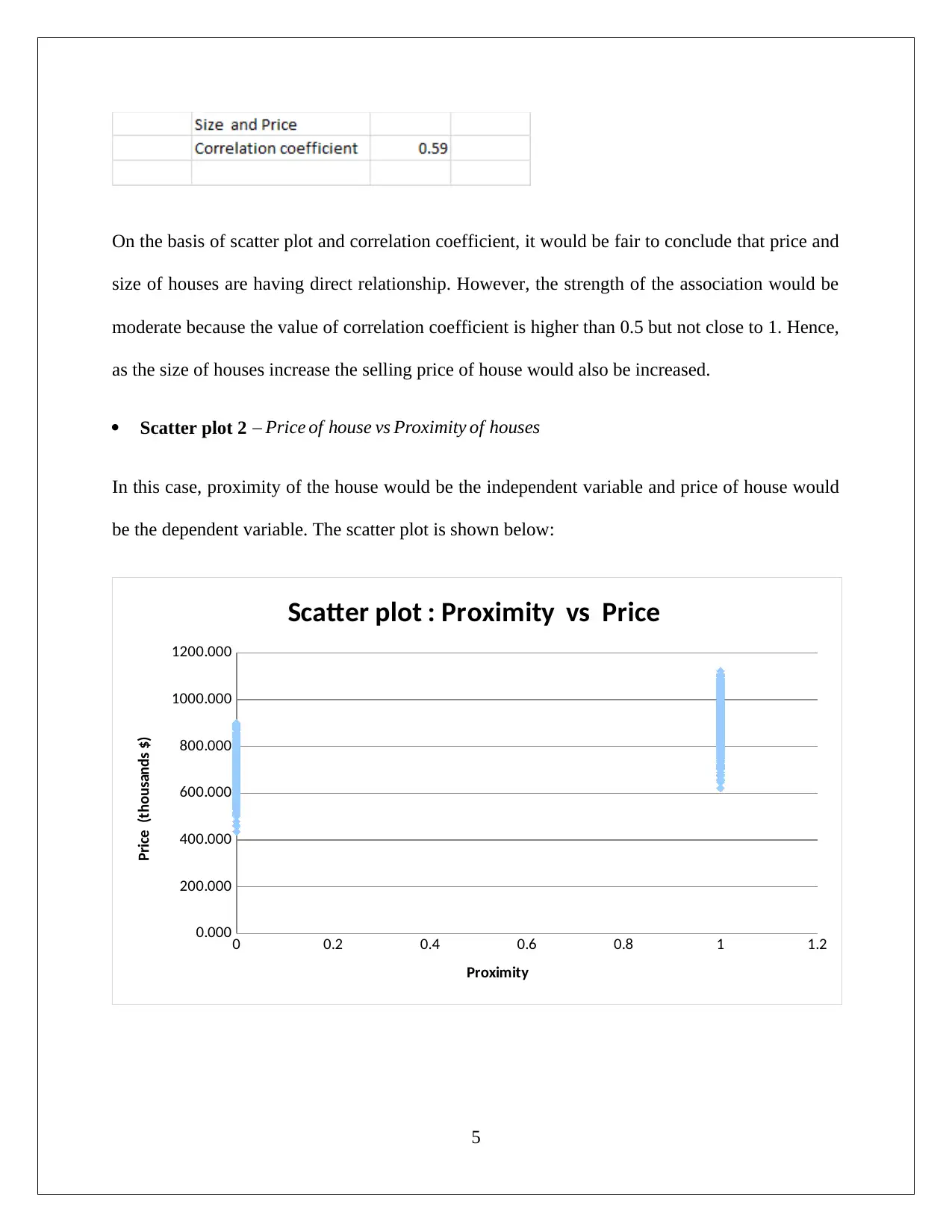
On the basis of scatter plot and correlation coefficient, it would be fair to conclude that price and
size of houses are having direct relationship. However, the strength of the association would be
moderate because the value of correlation coefficient is higher than 0.5 but not close to 1. Hence,
as the size of houses increase the selling price of house would also be increased.
 Scatter plot 2 – Price of house vs Proximity of houses
In this case, proximity of the house would be the independent variable and price of house would
be the dependent variable. The scatter plot is shown below:
0 0.2 0.4 0.6 0.8 1 1.2
0.000
200.000
400.000
600.000
800.000
1000.000
1200.000
Scatter plot : Proximity vs Price
Proximity
Price (thousands $)
5

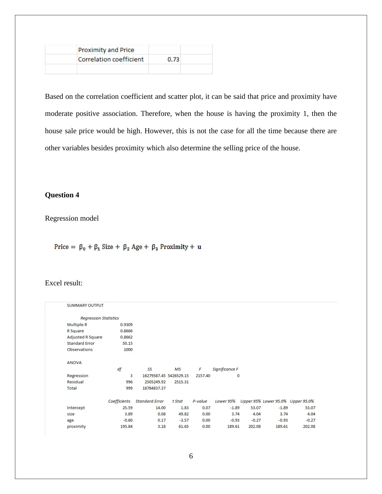
Based on the correlation coefficient and scatter plot, it can be said that price and proximity have
moderate positive association. Therefore, when the house is having the proximity 1, then the
house sale price would be high. However, this is not the case for all the time because there are
other variables besides proximity which also determine the selling price of the house.
Question 4
Regression model
Excel result:
6

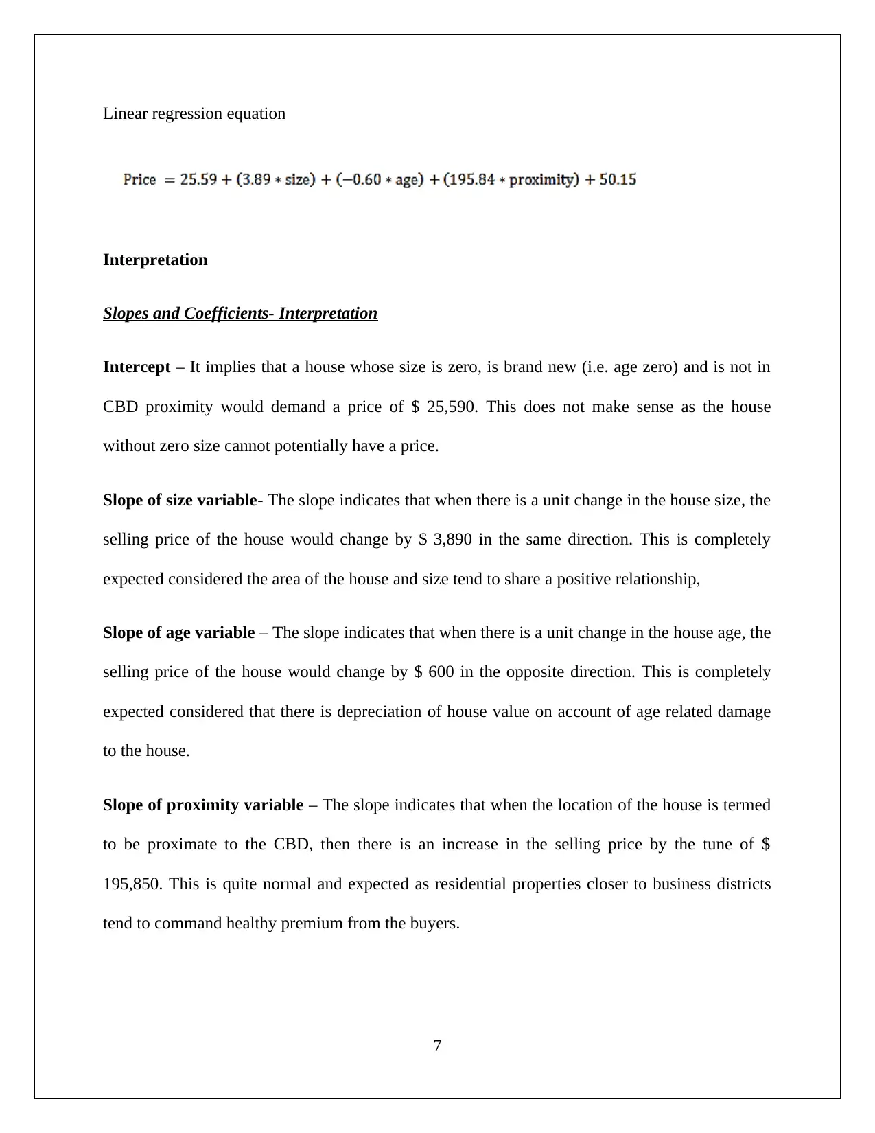
Linear regression equation
Interpretation
Slopes and Coefficients- Interpretation
Intercept – It implies that a house whose size is zero, is brand new (i.e. age zero) and is not in
CBD proximity would demand a price of $ 25,590. This does not make sense as the house
without zero size cannot potentially have a price.
Slope of size variable- The slope indicates that when there is a unit change in the house size, the
selling price of the house would change by $ 3,890 in the same direction. This is completely
expected considered the area of the house and size tend to share a positive relationship,
Slope of age variable – The slope indicates that when there is a unit change in the house age, the
selling price of the house would change by $ 600 in the opposite direction. This is completely
expected considered that there is depreciation of house value on account of age related damage
to the house.
Slope of proximity variable – The slope indicates that when the location of the house is termed
to be proximate to the CBD, then there is an increase in the selling price by the tune of $
195,850. This is quite normal and expected as residential properties closer to business districts
tend to command healthy premium from the buyers.
7

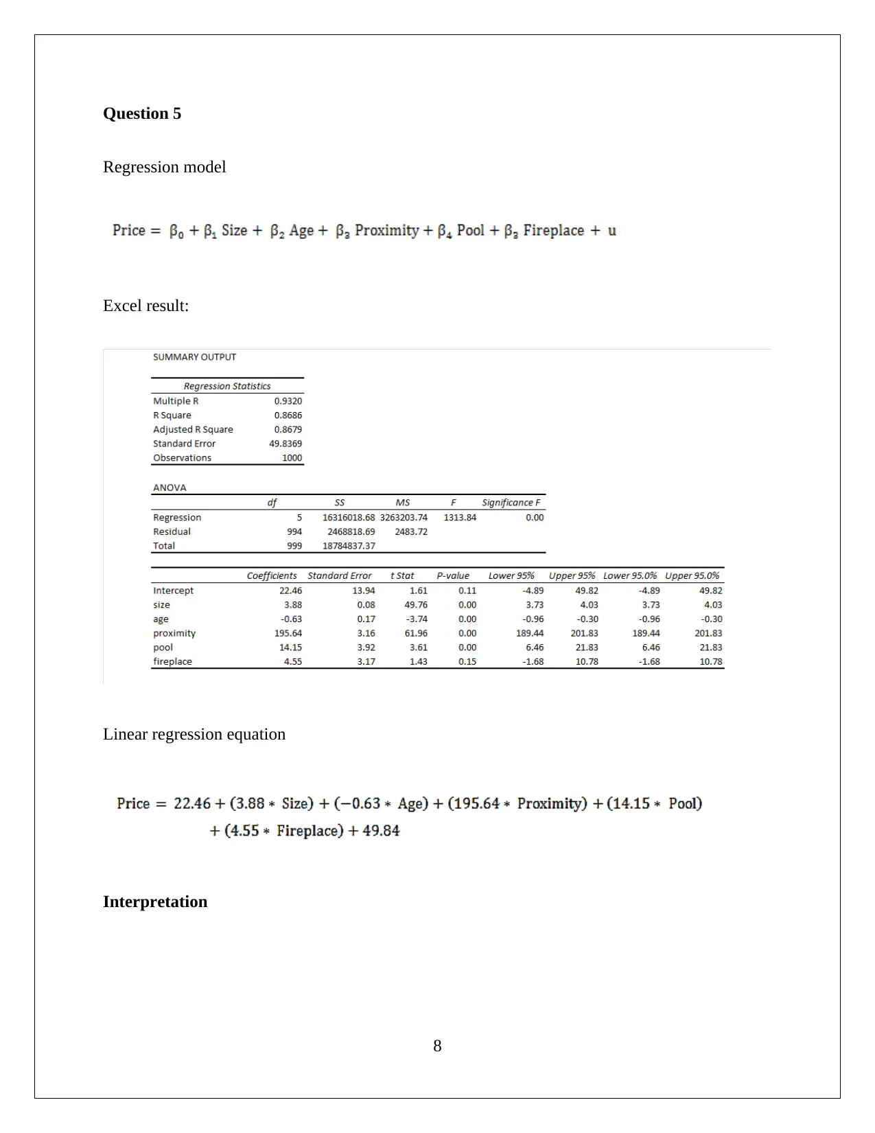
Question 5
Regression model
Excel result:
Linear regression equation
Interpretation
8

In the given model, there has been addition of two dummy variations, however with regards to
the model fit there has been no improvement. On the contrary, it seems that model fit has
worsened as highlighted from observations underlined below.
 The R2 (i.e. coefficient of determination) along with adjusted R2 have taken a lower value as
compared to the corresponding values in the earlier regression model which did not contain
the two dummy variables. This reflects lower ability of the independent variables to explain
respective changes in dependent variable or selling price.
 Besides, the ANOVA table which highlights the result of the F test also tends to hint at
worsening fit of model as the computed F statistic and the p value has shown a decline which
is a reflection of the lower significance of the given regression model in comparison with the
previous one.
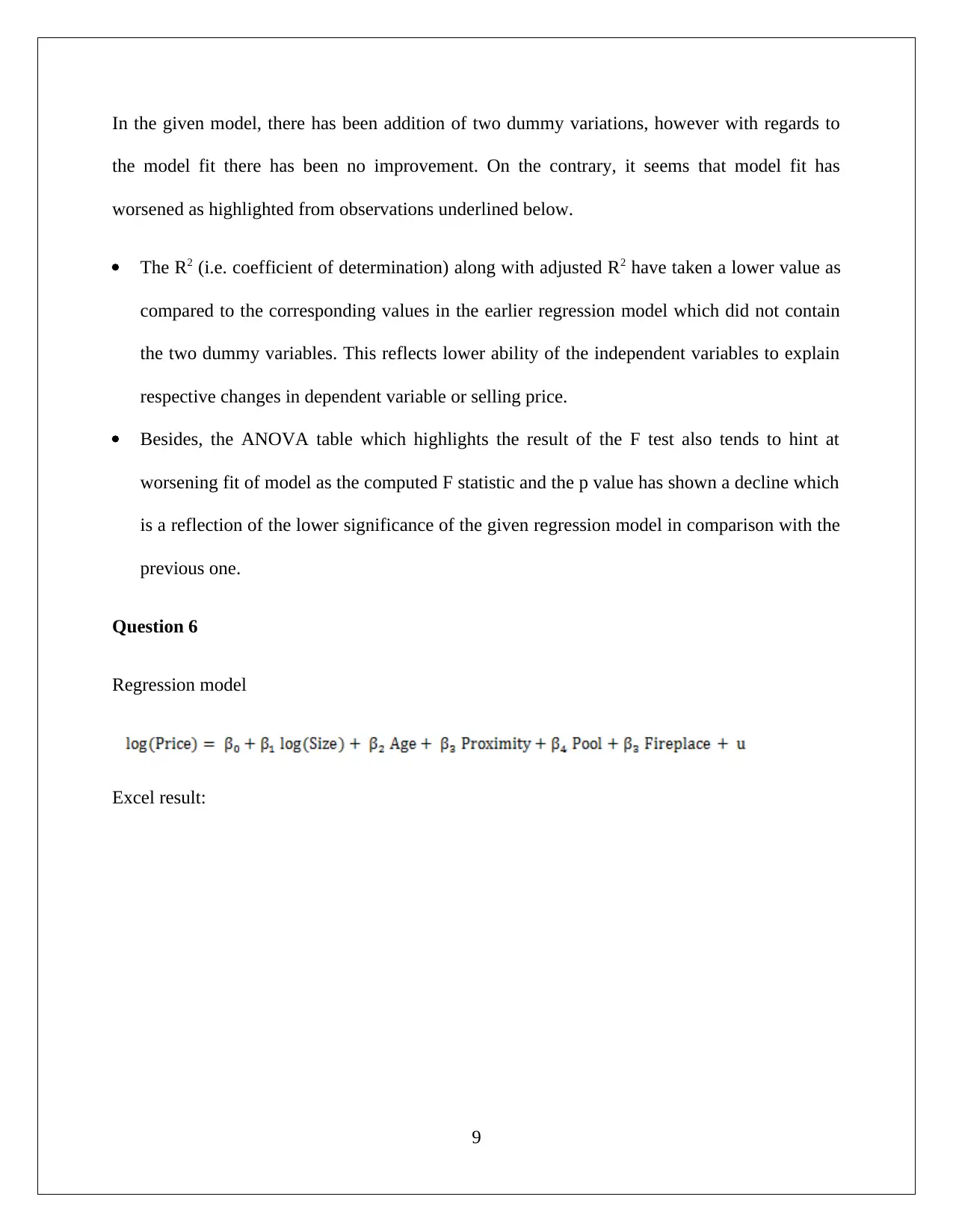
Question 6
Regression model
Excel result:
9

Linear regression equation
Interpretation
Requisite Coefficient Interpretation
β1 – This value indicates that a one unit change in the natural log of house size would produce a
0.8472 change in the price natural log in the same direction.
β4 – This value indicates that with the house having a swimming pool, there is an increase in the
price natural log to the tune of 0.0186. This highlights the fact that swimming pool presence
tends to attract higher valuation for the house.
10

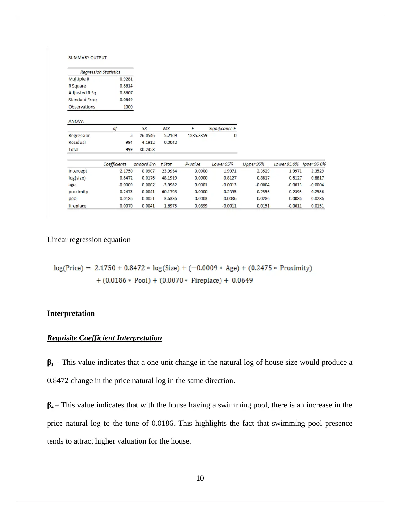
Question 7
Null hypothesis H0 : β5=0 i.e. slope coefficient of variable fireplace is equal to zero.
Alternative hypothesis H1 : β5 ≠ 0 i.e. slope coefficient of variable fireplace is not equal to zero.
The value of t stat is 1.6975 and the corresponding p value is 0.0899.
 Significance level=1 %
It can be seen that significance level is lower than p value and thus, null hypothesis would not be
rejected. Therefore, it would be concluded that slope coefficient of variable fireplace is assumed
to be equal to zero. Hence, fireplace does not create any statistical significant impact on the
selling price of the houses.
 Significance level=10 %
11

It can be seen that significance level is higher than p value and thus, null hypothesis would be
rejected. Therefore, it would be concluded that slope coefficient of variable fireplace is not equal
to zero. Hence, fireplace creates statistically significant impact on the selling price of the houses.
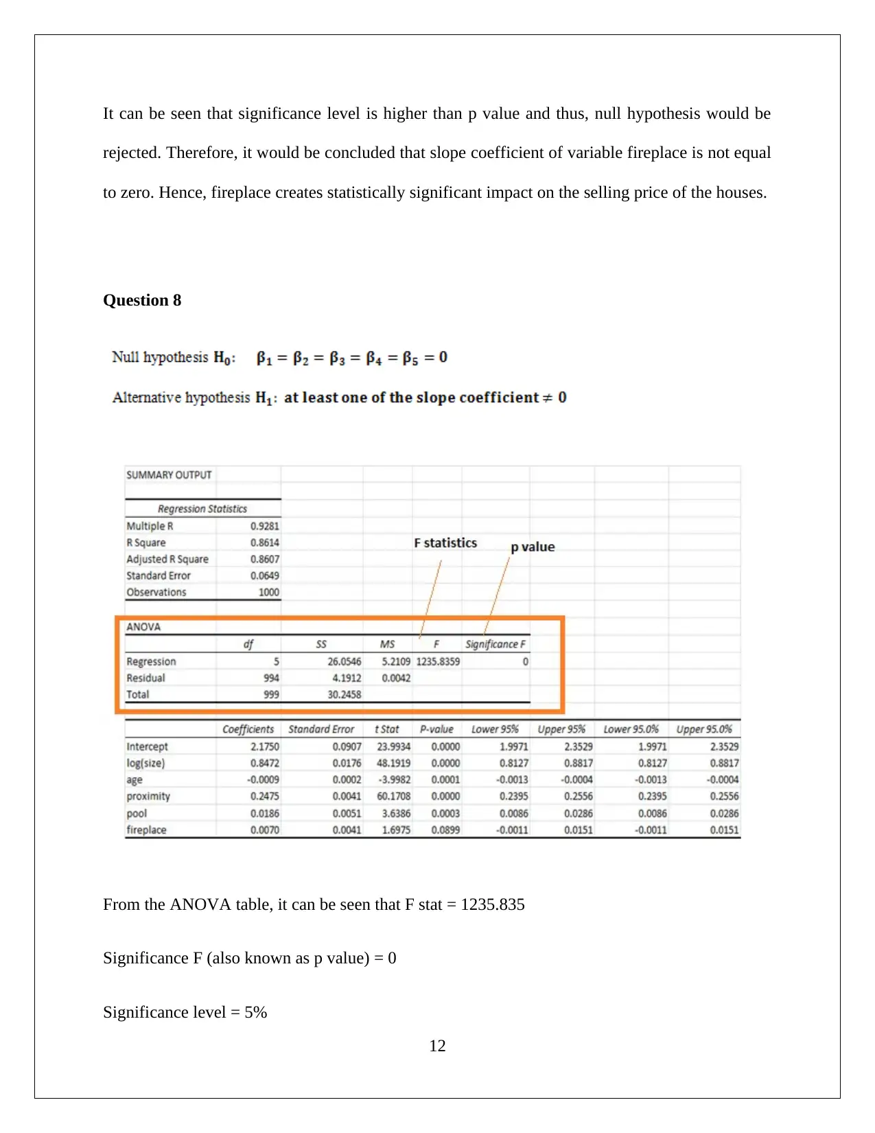
Question 8
From the ANOVA table, it can be seen that F stat = 1235.835
Significance F (also known as p value) = 0
Significance level = 5%
12

It can be seen that significance level is higher than p value and thus, null hypothesis would be
rejected. Therefore, it leads to the acceptance for alternative hypothesis. It would be concluded
that at least slope coefficient of among all the variable is statistically significant and not equal to
zero.
13