Statistics: Test for Difference in Blood Pressure, Time to Complete Exam, Reading Ability, and Cancer Grades

This document discusses statistical tests for difference in blood pressure, time to complete exam, reading ability, and cancer grades. It explains the appropriate statistical tests to use and provides the results obtained. The document also explores the relationship between variables and the significance of the findings.

Statistics
Statistics
Student name:
Instructor:
1 | P a g e

Statistics
NUMBER ONE
Test for the difference in blood pressure in mmHg taken while standing and while seated. The
appropriate statistical test to be run in this case is a paired sample t-test. This is so because two
datasets was obtained from the same sample. It is a “before and after” kind of data. Since paired
sample t-test is a parametric test there was need to verify the normality of the data we are dealing
with. There are various assumptions to be made before the parametric test is applied. The first
one is normality. The data is tested for normality since the parametric tests as mentioned earlier
are very sensitive to normality. Presence of outliers in a data affects the distribution of the data
hence making the data not to be normal. The outliers also affect the measures of central
tendencies such as the mean. There are various methods to ascertain normality of a distribution.
One of them is the use of histogram. The histogram will be able to present the distribution of the
data graphically so that it can be viewed or looked at and interpretations made with respect to the
shape of the histogram. It can be skewed to the left, right or normally distributed. When it is
skewed to the left, the curve on the histogram appears to have a long tail to the right. When it is
skewed to the right, the curve on the histogram appears to have a long tail to the left. In cases of
normal distribution, the curve appears to be bell-shaped. The other method to assess normality is
by the use of q-q plots. If the data points appear to cluster along the diagonal line on the plot,
then it means the data is normally distributed. If many points appear not to be along the diagonal
line then the data is not normally distributed. The other method to assess normality is by the use
of descriptive statistics under distribution. In this case we check the kurtosis values. For a
normally distributed data, the kurtosis value should be zero or towards zero. A histogram was
thus employed to establish the distribution. The graph is as shown below;
2 | P a g e

Statistics
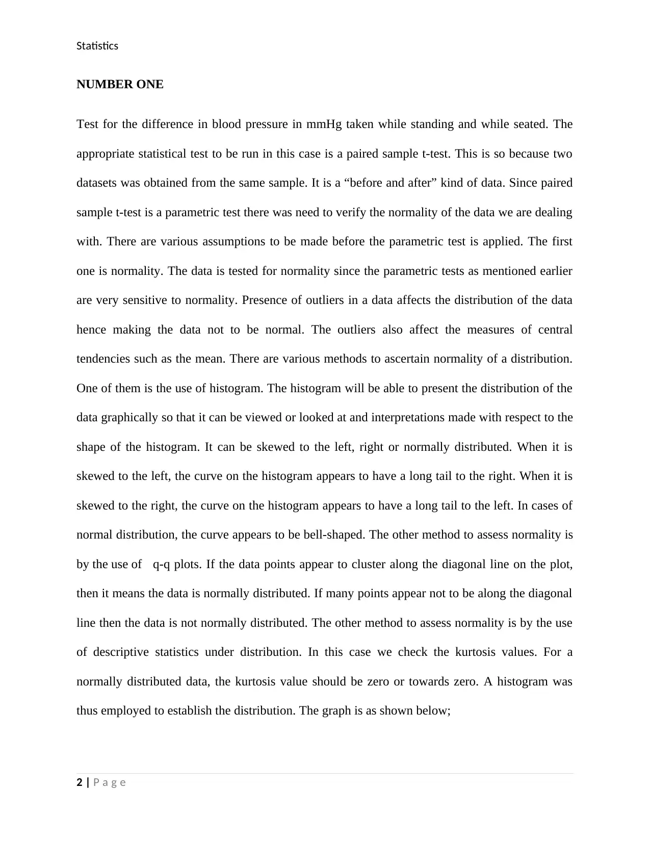
Histogram of standing BP
Figure 1
As can be observed from figure 1, the histograms show that the distribution of the blood pressure
while seated and standing are normally distributed. For a normal distribution, the normal curve
assumes a bell-shape. It is sometimes referred to as a symmetrical curve. It can be skewed to the
left, right or normally distributed. When it is skewed to the left, the curve on the histogram
appears to have a long tail to the right. When it is skewed to the right, the curve on the histogram
appears to have a long tail to the left. In cases of normal distribution, the curve appears to be
bell-shaped. Looking at the skewness in figure 1, it can be confirmed that the data was neither
skewed to the right nor to the left. It also has a low kurtosis since the peak is not high and sharp.
It is therefore confirmed that the paired sample t-test can be used to run the test.
3 | P a g e

Statistics
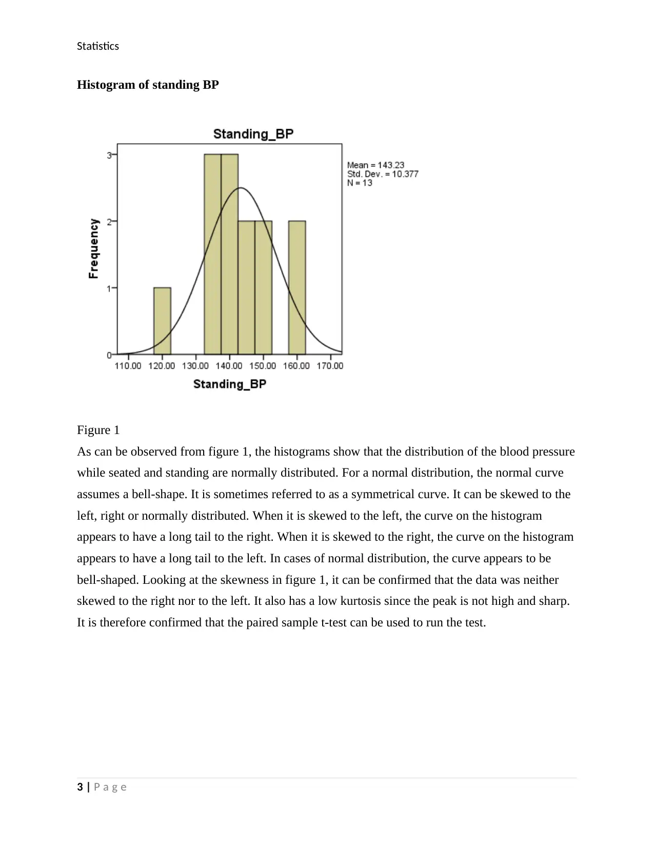
Histogram of seated BP
Figure 2
As can be observed from figure 2, the histograms show that the distribution of the blood pressure
while seated and standing are normally distributed. For a normal distribution, the normal curve
assumes a bell-shape. It is sometimes referred to as a symmetrical curve. It can be skewed to the
left, right or normally distributed. When it is skewed to the left, the curve on the histogram
appears to have a long tail to the right. When it is skewed to the right, the curve on the histogram
appears to have a long tail to the left. In cases of normal distribution, the curve appears to be
bell-shaped. Looking at the skewness in figure 2, it can be confirmed that the data was neither
skewed to the right nor to the left. It also has a low kurtosis since the peak is not high and sharp.
It is therefore confirmed that the paired sample t-test can be used to run the test.
Paired sample t-test
Hypothesis
H0: There is no difference in mean standing BP and seated BP.
H1: There is a significant difference in mean standing BP and seated BP.
4 | P a g e

Statistics
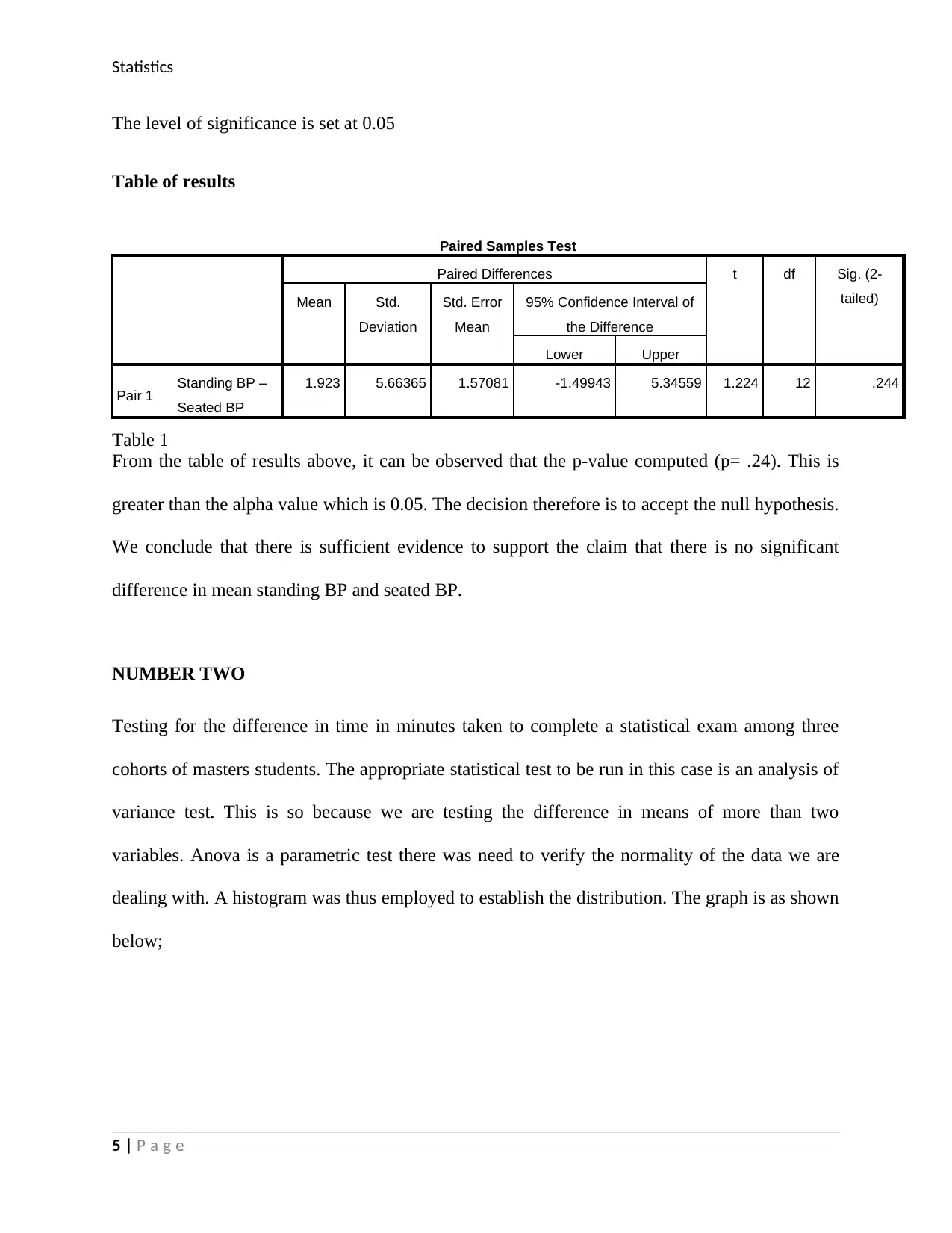
The level of significance is set at 0.05
Table of results
Paired Samples Test
Paired Differences t df Sig. (2-
tailed)Mean Std.
Deviation
Std. Error
Mean
95% Confidence Interval of
the Difference
Lower Upper
Pair 1 Standing BP –
Seated BP
1.923 5.66365 1.57081 -1.49943 5.34559 1.224 12 .244
Table 1
From the table of results above, it can be observed that the p-value computed (p= .24). This is
greater than the alpha value which is 0.05. The decision therefore is to accept the null hypothesis.
We conclude that there is sufficient evidence to support the claim that there is no significant
difference in mean standing BP and seated BP.
NUMBER TWO
Testing for the difference in time in minutes taken to complete a statistical exam among three
cohorts of masters students. The appropriate statistical test to be run in this case is an analysis of
variance test. This is so because we are testing the difference in means of more than two
variables. Anova is a parametric test there was need to verify the normality of the data we are
dealing with. A histogram was thus employed to establish the distribution. The graph is as shown
below;
5 | P a g e

Statistics
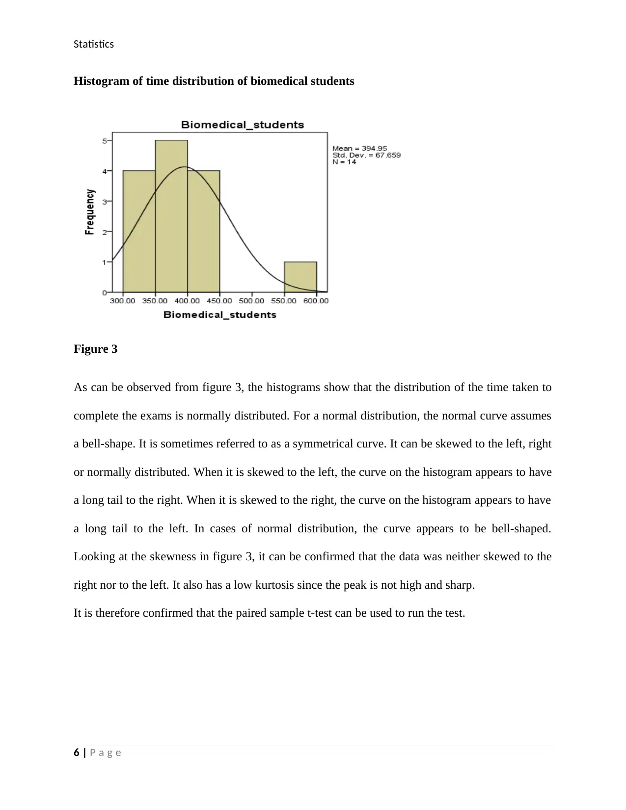
Histogram of time distribution of biomedical students
Figure 3
As can be observed from figure 3, the histograms show that the distribution of the time taken to
complete the exams is normally distributed. For a normal distribution, the normal curve assumes
a bell-shape. It is sometimes referred to as a symmetrical curve. It can be skewed to the left, right
or normally distributed. When it is skewed to the left, the curve on the histogram appears to have
a long tail to the right. When it is skewed to the right, the curve on the histogram appears to have
a long tail to the left. In cases of normal distribution, the curve appears to be bell-shaped.
Looking at the skewness in figure 3, it can be confirmed that the data was neither skewed to the
right nor to the left. It also has a low kurtosis since the peak is not high and sharp.
It is therefore confirmed that the paired sample t-test can be used to run the test.
6 | P a g e

Statistics
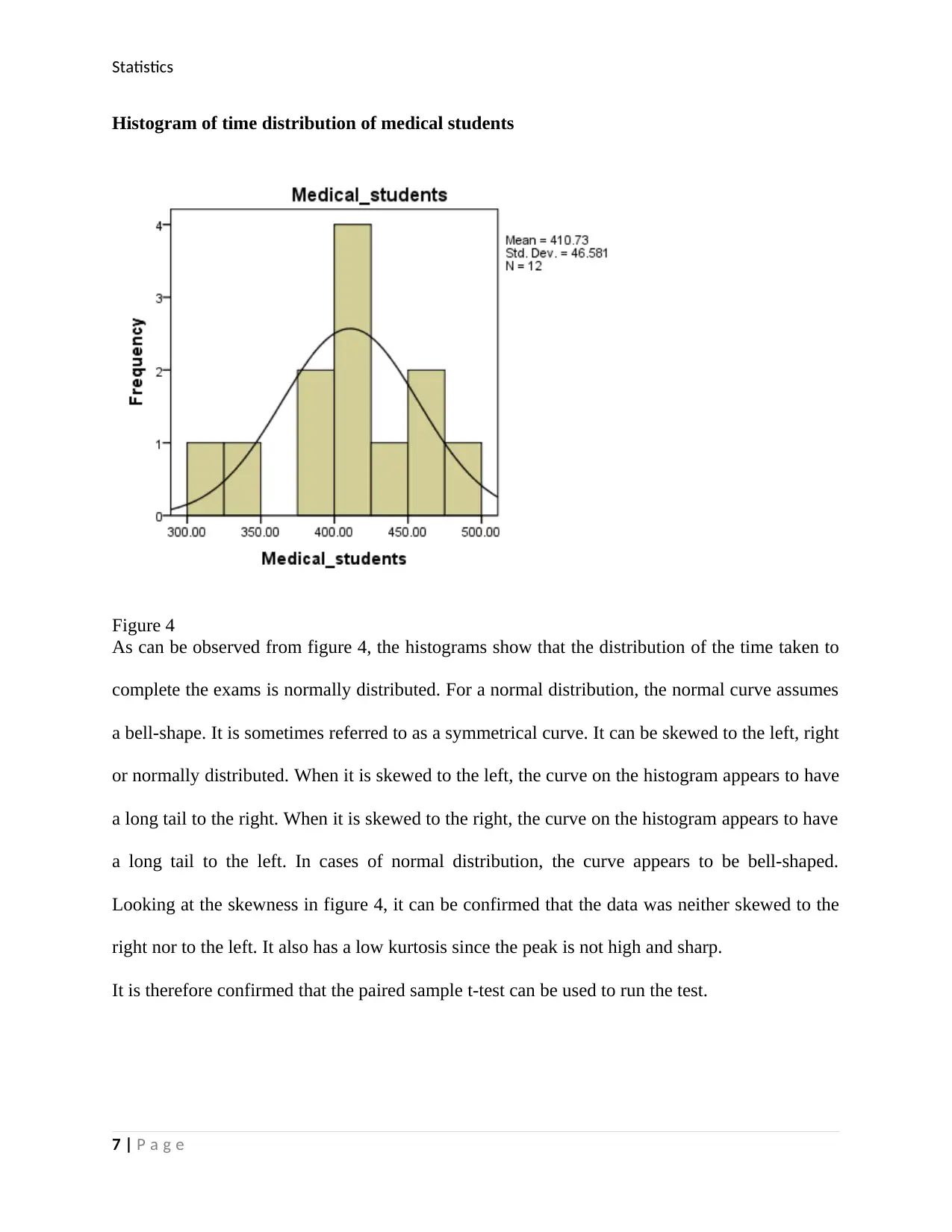
Histogram of time distribution of medical students
Figure 4
As can be observed from figure 4, the histograms show that the distribution of the time taken to
complete the exams is normally distributed. For a normal distribution, the normal curve assumes
a bell-shape. It is sometimes referred to as a symmetrical curve. It can be skewed to the left, right
or normally distributed. When it is skewed to the left, the curve on the histogram appears to have
a long tail to the right. When it is skewed to the right, the curve on the histogram appears to have
a long tail to the left. In cases of normal distribution, the curve appears to be bell-shaped.
Looking at the skewness in figure 4, it can be confirmed that the data was neither skewed to the
right nor to the left. It also has a low kurtosis since the peak is not high and sharp.
It is therefore confirmed that the paired sample t-test can be used to run the test.
7 | P a g e

Statistics
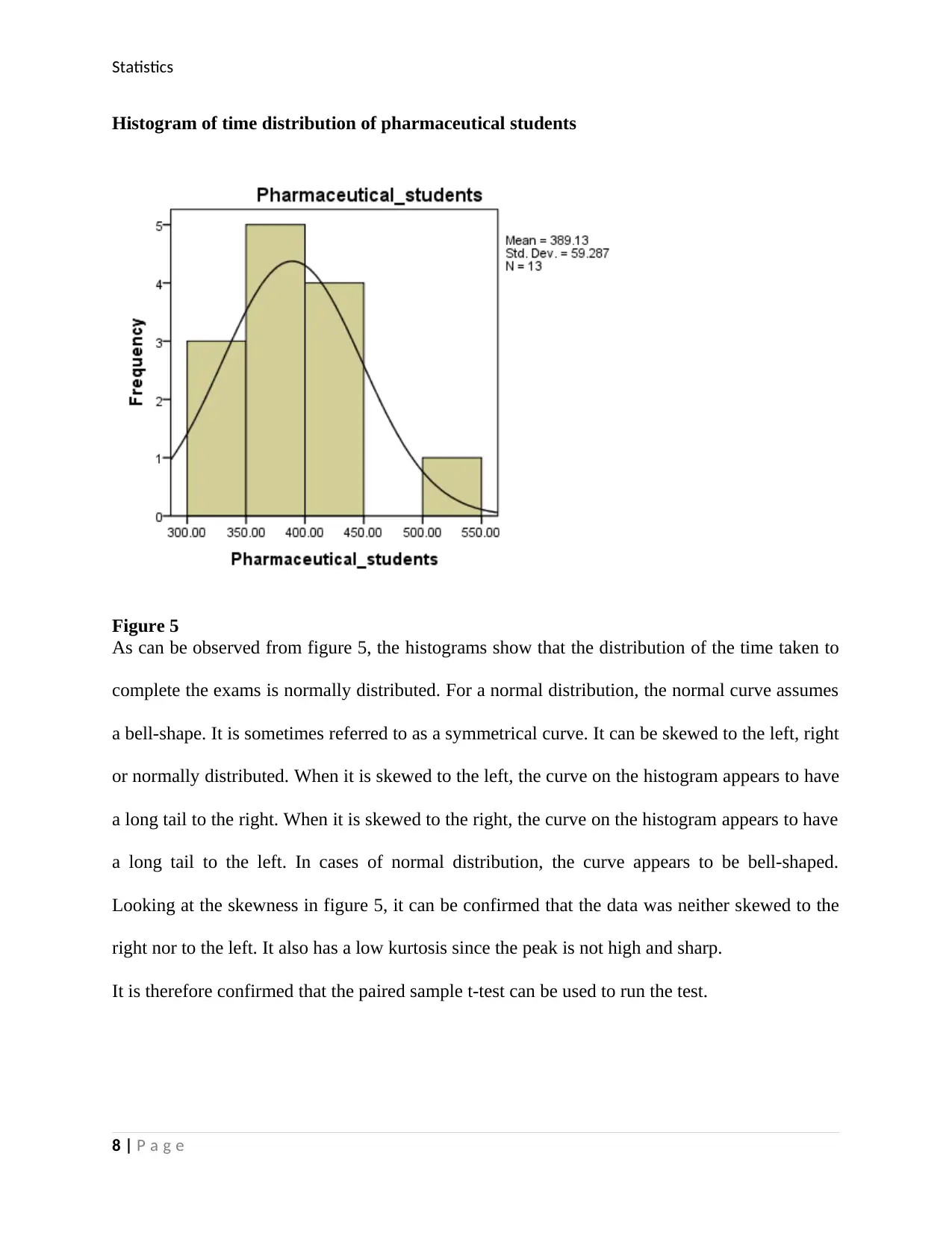
Histogram of time distribution of pharmaceutical students
Figure 5
As can be observed from figure 5, the histograms show that the distribution of the time taken to
complete the exams is normally distributed. For a normal distribution, the normal curve assumes
a bell-shape. It is sometimes referred to as a symmetrical curve. It can be skewed to the left, right
or normally distributed. When it is skewed to the left, the curve on the histogram appears to have
a long tail to the right. When it is skewed to the right, the curve on the histogram appears to have
a long tail to the left. In cases of normal distribution, the curve appears to be bell-shaped.
Looking at the skewness in figure 5, it can be confirmed that the data was neither skewed to the
right nor to the left. It also has a low kurtosis since the peak is not high and sharp.
It is therefore confirmed that the paired sample t-test can be used to run the test.
8 | P a g e

Statistics
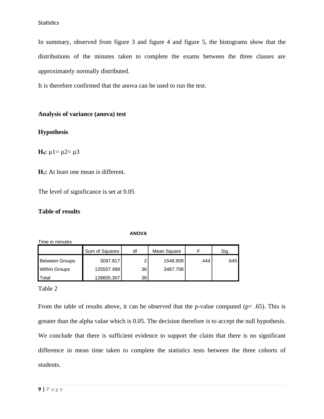
In summary, observed from figure 3 and figure 4 and figure 5, the histograms show that the
distributions of the minutes taken to complete the exams between the three classes are
approximately normally distributed.
It is therefore confirmed that the anova can be used to run the test.
Analysis of variance (anova) test
Hypothesis
H0: μ1= μ2= μ3
H1: At least one mean is different.
The level of significance is set at 0.05
Table of results
ANOVA
Time in minutes
Sum of Squares df Mean Square F Sig.
Between Groups 3097.817 2 1548.909 .444 .645
Within Groups 125557.489 36 3487.708
Total 128655.307 38
Table 2
From the table of results above, it can be observed that the p-value computed (p= .65). This is
greater than the alpha value which is 0.05. The decision therefore is to accept the null hypothesis.
We conclude that there is sufficient evidence to support the claim that there is no significant
difference in mean time taken to complete the statistics tests between the three cohorts of
students.
9 | P a g e

Statistics
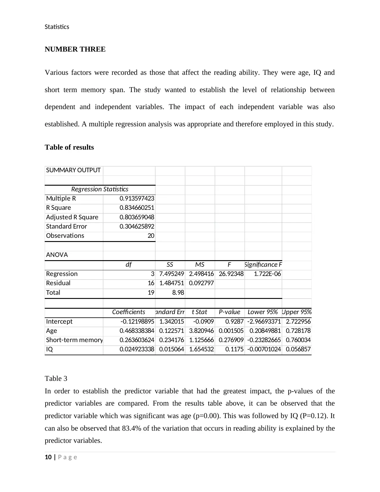
NUMBER THREE
Various factors were recorded as those that affect the reading ability. They were age, IQ and
short term memory span. The study wanted to establish the level of relationship between
dependent and independent variables. The impact of each independent variable was also
established. A multiple regression analysis was appropriate and therefore employed in this study.
Table of results
SUMMARY OUTPUT
Regression Statistics
Multiple R 0.913597423
R Square 0.834660251
Adjusted R Square 0.803659048
Standard Error 0.304625892
Observations 20
ANOVA
df SS MS F Significance F
Regression 3 7.495249 2.498416 26.92348 1.722E-06
Residual 16 1.484751 0.092797
Total 19 8.98
Coefficients Standard Error t Stat P-value Lower 95% Upper 95%
Intercept -0.12198895 1.342015 -0.0909 0.9287 -2.96693371 2.722956
Age 0.468338384 0.122571 3.820946 0.001505 0.20849881 0.728178
Short-term memory span 0.263603624 0.234176 1.125666 0.276909 -0.23282665 0.760034
IQ 0.024923338 0.015064 1.654532 0.1175 -0.00701024 0.056857
Table 3
In order to establish the predictor variable that had the greatest impact, the p-values of the
predictor variables are compared. From the results table above, it can be observed that the
predictor variable which was significant was age (p=0.00). This was followed by IQ (P=0.12). It
can also be observed that 83.4% of the variation that occurs in reading ability is explained by the
predictor variables.
10 | P a g e

Statistics
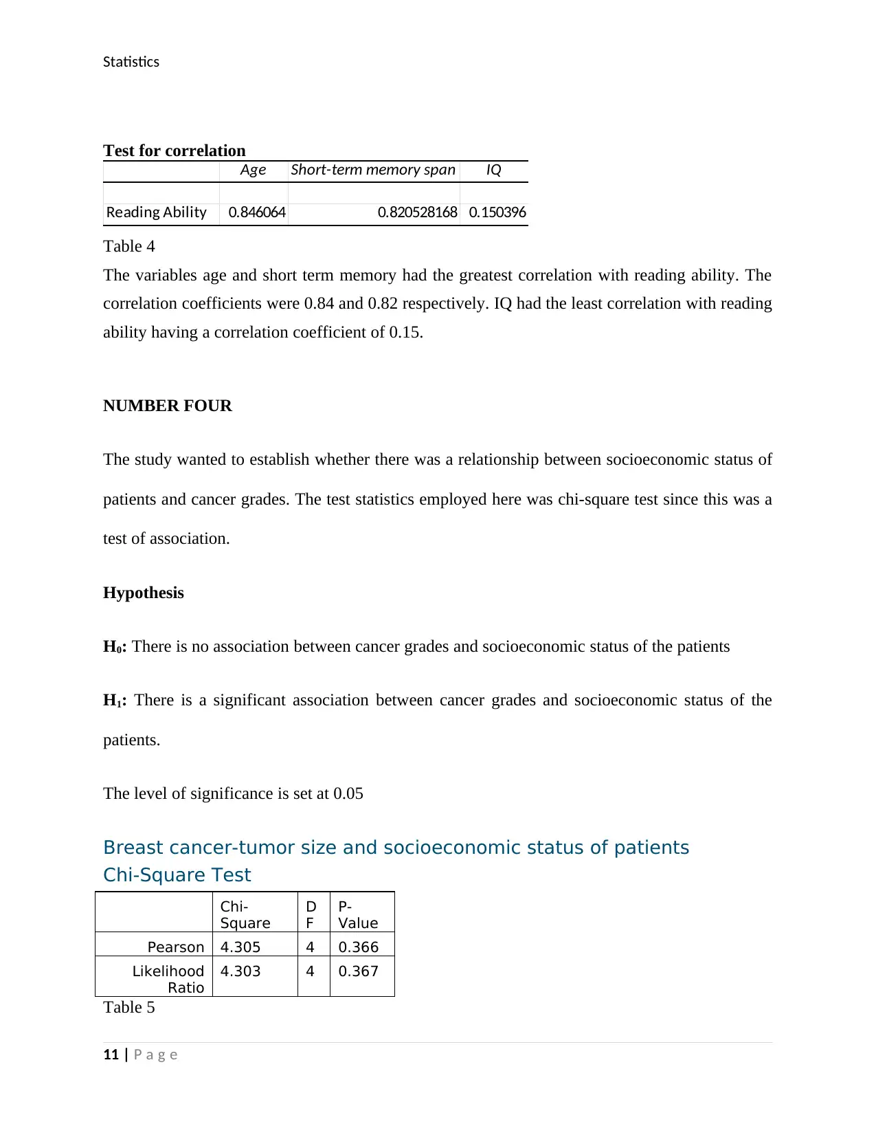
Test for correlation
Age Short-term memory span IQ
Reading Ability 0.846064 0.820528168 0.150396
Table 4
The variables age and short term memory had the greatest correlation with reading ability. The
correlation coefficients were 0.84 and 0.82 respectively. IQ had the least correlation with reading
ability having a correlation coefficient of 0.15.
NUMBER FOUR
The study wanted to establish whether there was a relationship between socioeconomic status of
patients and cancer grades. The test statistics employed here was chi-square test since this was a
test of association.
Hypothesis
H0: There is no association between cancer grades and socioeconomic status of the patients
H1: There is a significant association between cancer grades and socioeconomic status of the
patients.
The level of significance is set at 0.05
Breast cancer-tumor size and socioeconomic status of patients
Chi-Square Test
Chi-
Square
D
F
P-
Value
Pearson 4.305 4 0.366
Likelihood
Ratio
4.303 4 0.367
Table 5
11 | P a g e

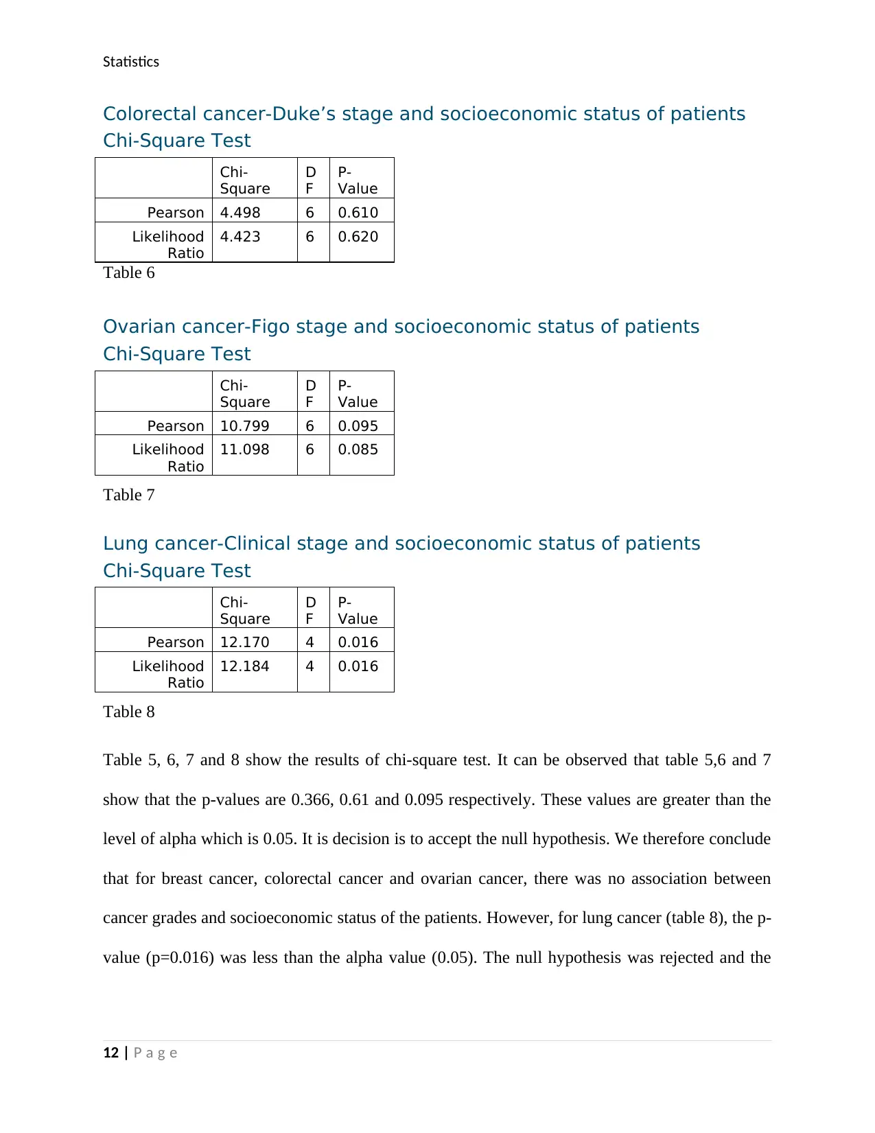
Statistics
Colorectal cancer-Duke’s stage and socioeconomic status of patients
Chi-Square Test
Chi-
Square
D
F
P-
Value
Pearson 4.498 6 0.610
Likelihood
Ratio
4.423 6 0.620
Table 6
Ovarian cancer-Figo stage and socioeconomic status of patients
Chi-Square Test
Chi-
Square
D
F
P-
Value
Pearson 10.799 6 0.095
Likelihood
Ratio
11.098 6 0.085
Table 7
Lung cancer-Clinical stage and socioeconomic status of patients
Chi-Square Test
Chi-
Square
D
F
P-
Value
Pearson 12.170 4 0.016
Likelihood
Ratio
12.184 4 0.016
Table 8
Table 5, 6, 7 and 8 show the results of chi-square test. It can be observed that table 5,6 and 7
show that the p-values are 0.366, 0.61 and 0.095 respectively. These values are greater than the
level of alpha which is 0.05. It is decision is to accept the null hypothesis. We therefore conclude
that for breast cancer, colorectal cancer and ovarian cancer, there was no association between
cancer grades and socioeconomic status of the patients. However, for lung cancer (table 8), the p-
value (p=0.016) was less than the alpha value (0.05). The null hypothesis was rejected and the
12 | P a g e

Statistics
alternative accepted. The conclusion was that there is a significant association between cancer
grades and socioeconomic status of the patients.
13 | P a g e