Statistics: Analysis of Revenue and Visits for QA Company
VerifiedAdded on 2023/03/30
|16
|2641
|218
AI Summary
This study analyzes the revenue and visits data for QA Company over a period of time. It examines the correlation between revenue and pounds sold, as well as revenue and visits. The findings suggest that there is a strong correlation between revenue and pounds sold, while there is no significant correlation between revenue and visits.
Contribute Materials
Your contribution can guide someone’s learning journey. Share your
documents today.

Statistics
Statistics
Student name:
Tutor name:
1 | P a g e
Statistics
Student name:
Tutor name:
1 | P a g e
Secure Best Marks with AI Grader
Need help grading? Try our AI Grader for instant feedback on your assignments.
Statistics
Executive summary
QA is a company that deals in alloys. It sells its products to customers on request and
specification and also sells to wholesalers. It has curved its niche so well in this area that it is
well renowned. In the past two years, many companies have been coming up which produce the
same products as QA thus heightening competition. For this reason the company created a
website so as to better understand its customer needs and also widen its market. Information
collected from the website over a period of about one year was analyzed and findings presented
in form of tables and graphs. The results showed that there was no significant increase in the
amount of revenue despite more visits to the website. The study therefore recommended to the
management of QA to come up with other marketing strategies as the website was not doing
much to increase sales and hence revenue.
2 | P a g e
Statistics
Question 1
Unique visits to the QA website in line with weeks
May 25 - May 31
Jun 15 - Jun 21
Jul 6 - Jul 12
Jul 27 - Aug 2
Aug 17 - Aug 23
Sep 7 - Sep 13
Sep 28 - Oct 4
Oct 19 - Oct 25
Nov 9 - Nov 15
Nov 30 - Dec 6
Dec 21 - Dec 27
Jan 11 - Jan 17
Feb 1 - Feb 7
Feb 22 - Feb 28
Mar 15 - Mar 21
Apr 5 - Apr 11
Apr 26 - May 2
May 17 - May 23
Jun 7 - Jun 13
Jun 28 - Jul 4
Jul 19 - Jul 25
Aug 9 - Aug 15
0
500
1,000
1,500
2,000
2,500
3,000
3,500
4,000
Unique Visits to the QA
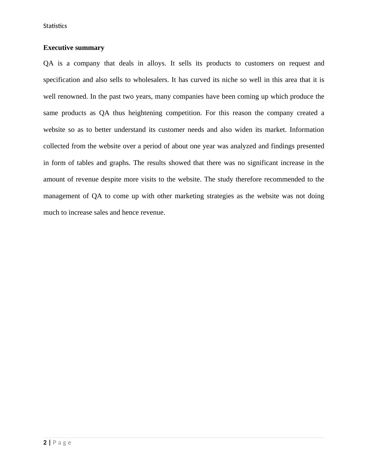
Fig. 1
The chart proven above (fig. 1) displays the distribution of unique visits for the length from 25th
May additionally, 2008 to fifteenth August 2009. From the start of the period, the weekly precise
visits decreased till around January 2009 while it commenced increasing till the month of
February as may be discovered from the graph. After the month of February, the range of
particular visits reduces normally to the end.
Distribution of revenue every week
3 | P a g e
Statistics
May 25 - May 31
Jun 22 - Jun 28
Jul 20 - Jul 26
Aug 17 - Aug 23
Sep 14 - Sep 20
Oct 12 - Oct 18
Nov 9 - Nov 15
Dec 7 - Dec 13
Jan 4 - Jan 10
Feb 1 - Feb 7
Mar 1 - Mar 7
Mar 29 - Apr 4
Apr 26 - May 2
May 24 - May 30
Jun 21 - Jun 27
Jul 19 - Jul 25
Aug 16 - Aug 22
$0
$100,000
$200,000
$300,000
$400,000
$500,000
$600,000
$700,000
$800,000
$900,000
$1,000,000
Fig. 2. Revenue frequency
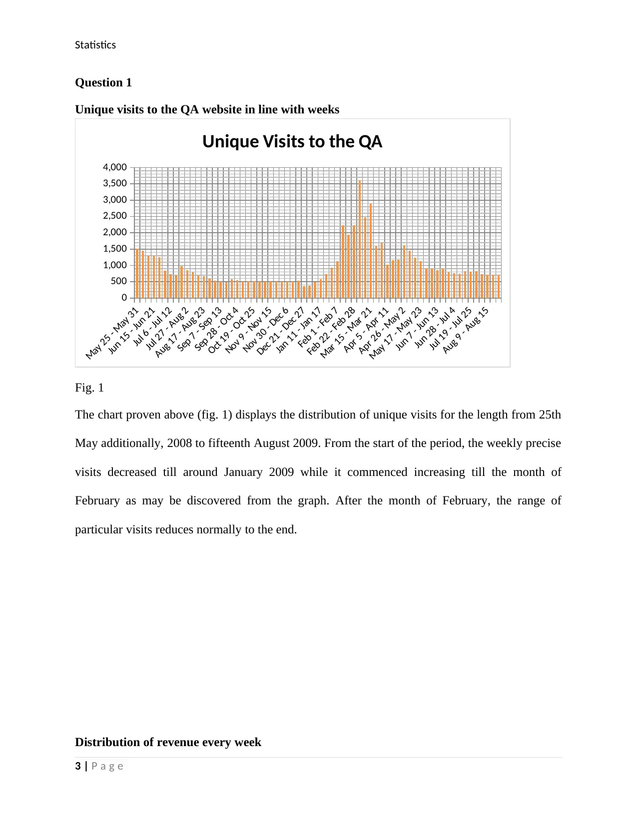
Fig. 2
Revenue quantity every week for the company from the beginning to the end of the period is
seen to stay generally the same save for few weeks which had more revenue.
Distribution of profit every week
May 25 - May 31
Jun 22 - Jun 28
Jul 20 - Jul 26
Aug 17 - Aug 23
Sep 14 - Sep 20
Oct 12 - Oct 18
Nov 9 - Nov 15
Dec 7 - Dec 13
Jan 4 - Jan 10
Feb 1 - Feb 7
Mar 1 - Mar 7
Mar 29 - Apr 4
Apr 26 - May 2
May 24 - May 30
Jun 21 - Jun 27
Jul 19 - Jul 25
Aug 16 - Aug 22
$0
$50,000
$100,000
$150,000
$200,000
$250,000
$300,000
Fig. 3. Profit over time per week
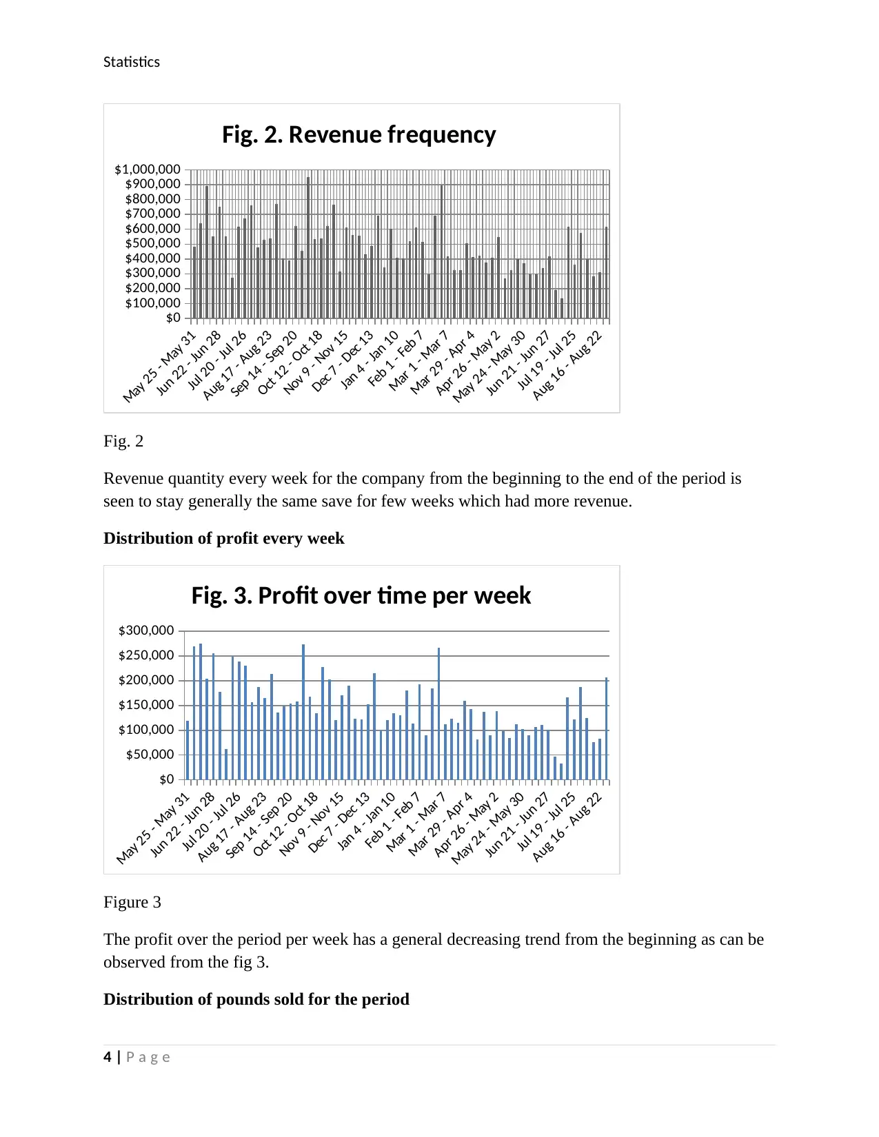
Figure 3
The profit over the period per week has a general decreasing trend from the beginning as can be
observed from the fig 3.
Distribution of pounds sold for the period
4 | P a g e
May 25 - May 31
Jun 22 - Jun 28
Jul 20 - Jul 26
Aug 17 - Aug 23
Sep 14 - Sep 20
Oct 12 - Oct 18
Nov 9 - Nov 15
Dec 7 - Dec 13
Jan 4 - Jan 10
Feb 1 - Feb 7
Mar 1 - Mar 7
Mar 29 - Apr 4
Apr 26 - May 2
May 24 - May 30
Jun 21 - Jun 27
Jul 19 - Jul 25
Aug 16 - Aug 22
$0
$100,000
$200,000
$300,000
$400,000
$500,000
$600,000
$700,000
$800,000
$900,000
$1,000,000
Fig. 2. Revenue frequency
Fig. 2
Revenue quantity every week for the company from the beginning to the end of the period is
seen to stay generally the same save for few weeks which had more revenue.
Distribution of profit every week
May 25 - May 31
Jun 22 - Jun 28
Jul 20 - Jul 26
Aug 17 - Aug 23
Sep 14 - Sep 20
Oct 12 - Oct 18
Nov 9 - Nov 15
Dec 7 - Dec 13
Jan 4 - Jan 10
Feb 1 - Feb 7
Mar 1 - Mar 7
Mar 29 - Apr 4
Apr 26 - May 2
May 24 - May 30
Jun 21 - Jun 27
Jul 19 - Jul 25
Aug 16 - Aug 22
$0
$50,000
$100,000
$150,000
$200,000
$250,000
$300,000
Fig. 3. Profit over time per week
Figure 3
The profit over the period per week has a general decreasing trend from the beginning as can be
observed from the fig 3.
Distribution of pounds sold for the period
4 | P a g e
Secure Best Marks with AI Grader
Need help grading? Try our AI Grader for instant feedback on your assignments.
Statistics
May 25 - May 31
Jun 22 - Jun 28
Jul 20 - Jul 26
Aug 17 - Aug 23
Sep 14 - Sep 20
Oct 12 - Oct 18
Nov 9 - Nov 15
Dec 7 - Dec 13
Jan 4 - Jan 10
Feb 1 - Feb 7
Mar 1 - Mar 7
Mar 29 - Apr 4
Apr 26 - May 2
May 24 - May 30
Jun 21 - Jun 27
Jul 19 - Jul 25
Aug 16 - Aug 22
0
5,000
10,000
15,000
20,000
25,000
30,000
35,000
Fig. 4. Pounds Sold
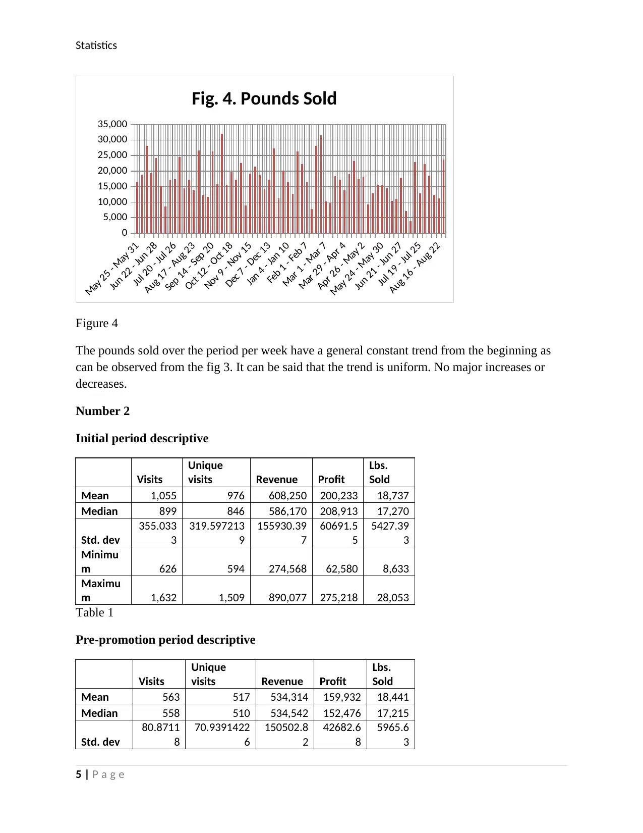
Figure 4
The pounds sold over the period per week have a general constant trend from the beginning as
can be observed from the fig 3. It can be said that the trend is uniform. No major increases or
decreases.
Number 2
Initial period descriptive
Visits
Unique
visits Revenue Profit
Lbs.
Sold
Mean 1,055 976 608,250 200,233 18,737
Median 899 846 586,170 208,913 17,270
Std. dev
355.033
3
319.597213
9
155930.39
7
60691.5
5
5427.39
3
Minimu
m 626 594 274,568 62,580 8,633
Maximu
m 1,632 1,509 890,077 275,218 28,053
Table 1
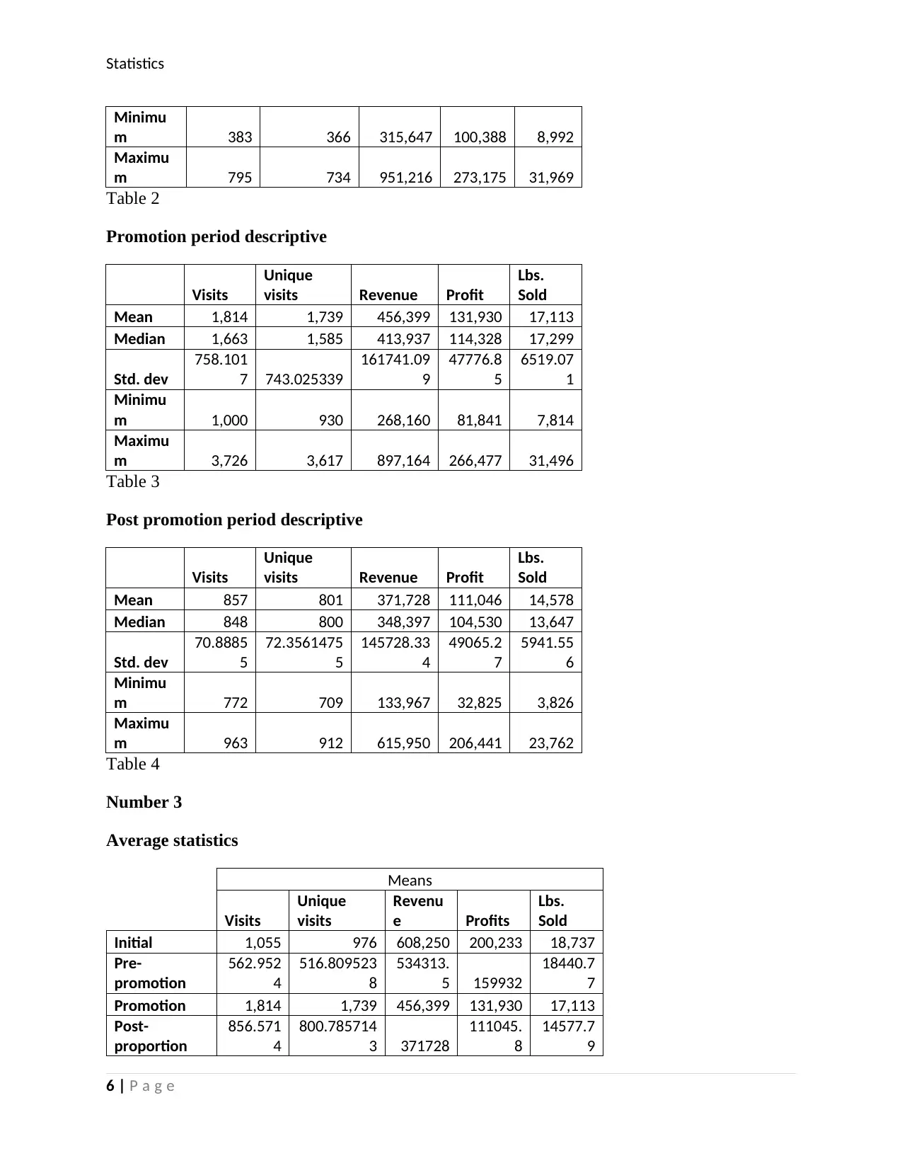
Pre-promotion period descriptive
Visits
Unique
visits Revenue Profit
Lbs.
Sold
Mean 563 517 534,314 159,932 18,441
Median 558 510 534,542 152,476 17,215
Std. dev
80.8711
8
70.9391422
6
150502.8
2
42682.6
8
5965.6
3
5 | P a g e
Statistics
Minimu
m 383 366 315,647 100,388 8,992
Maximu
m 795 734 951,216 273,175 31,969
Table 2
Promotion period descriptive
Visits
Unique
visits Revenue Profit
Lbs.
Sold
Mean 1,814 1,739 456,399 131,930 17,113
Median 1,663 1,585 413,937 114,328 17,299
Std. dev
758.101
7 743.025339
161741.09
9
47776.8
5
6519.07
1
Minimu
m 1,000 930 268,160 81,841 7,814
Maximu
m 3,726 3,617 897,164 266,477 31,496
Table 3
Post promotion period descriptive
Visits
Unique
visits Revenue Profit
Lbs.
Sold
Mean 857 801 371,728 111,046 14,578
Median 848 800 348,397 104,530 13,647
Std. dev
70.8885
5
72.3561475
5
145728.33
4
49065.2
7
5941.55
6
Minimu
m 772 709 133,967 32,825 3,826
Maximu
m 963 912 615,950 206,441 23,762
Table 4
Number 3
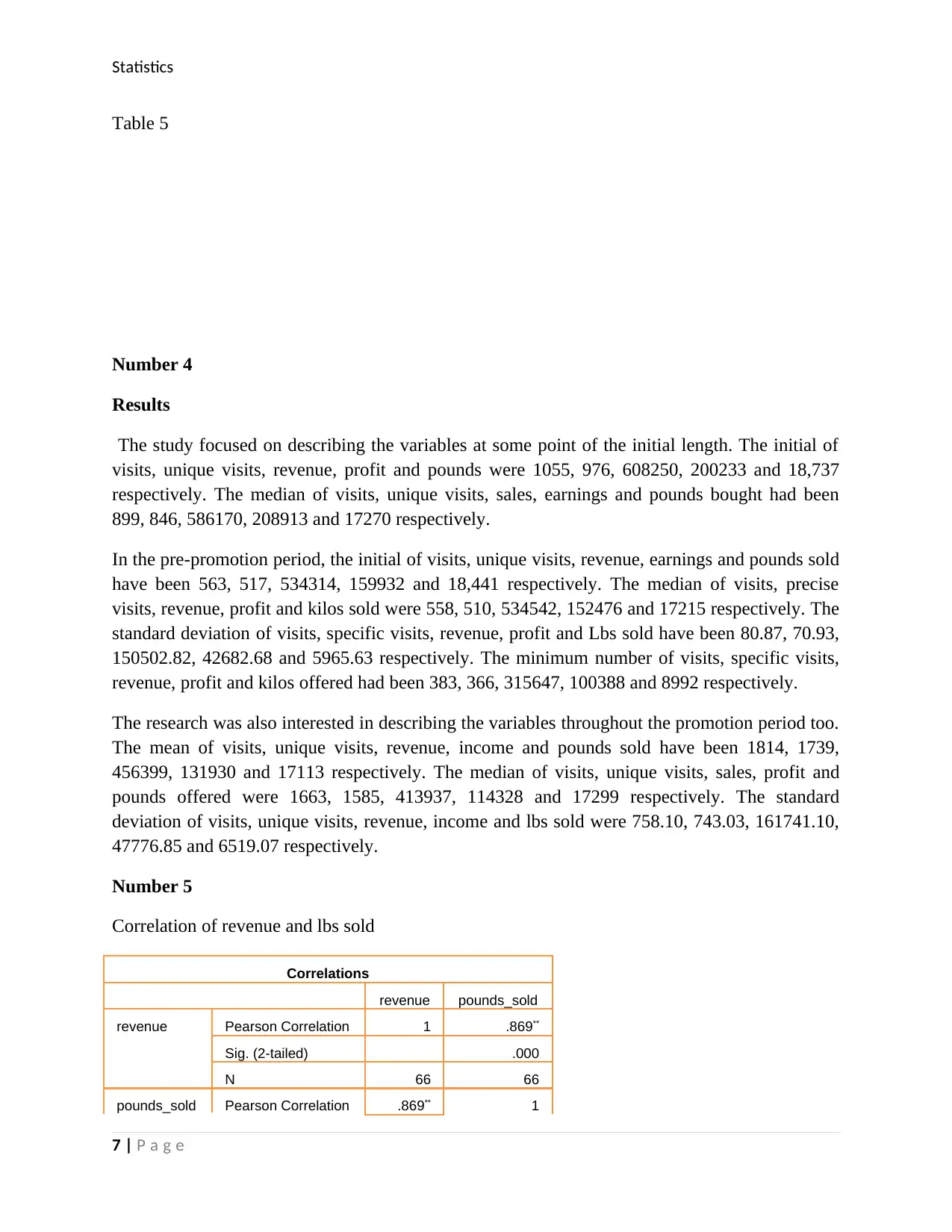
Average statistics
Means
Visits
Unique
visits
Revenu
e Profits
Lbs.
Sold
Initial 1,055 976 608,250 200,233 18,737
Pre-
promotion
562.952
4
516.809523
8
534313.
5 159932
18440.7
7
Promotion 1,814 1,739 456,399 131,930 17,113
Post-
proportion
856.571
4
800.785714
3 371728
111045.
8
14577.7
9
6 | P a g e
Minimu
m 383 366 315,647 100,388 8,992
Maximu
m 795 734 951,216 273,175 31,969
Table 2
Promotion period descriptive
Visits
Unique
visits Revenue Profit
Lbs.
Sold
Mean 1,814 1,739 456,399 131,930 17,113
Median 1,663 1,585 413,937 114,328 17,299
Std. dev
758.101
7 743.025339
161741.09
9
47776.8
5
6519.07
1
Minimu
m 1,000 930 268,160 81,841 7,814
Maximu
m 3,726 3,617 897,164 266,477 31,496
Table 3
Post promotion period descriptive
Visits
Unique
visits Revenue Profit
Lbs.
Sold
Mean 857 801 371,728 111,046 14,578
Median 848 800 348,397 104,530 13,647
Std. dev
70.8885
5
72.3561475
5
145728.33
4
49065.2
7
5941.55
6
Minimu
m 772 709 133,967 32,825 3,826
Maximu
m 963 912 615,950 206,441 23,762
Table 4
Number 3
Average statistics
Means
Visits
Unique
visits
Revenu
e Profits
Lbs.
Sold
Initial 1,055 976 608,250 200,233 18,737
Pre-
promotion
562.952
4
516.809523
8
534313.
5 159932
18440.7
7
Promotion 1,814 1,739 456,399 131,930 17,113
Post-
proportion
856.571
4
800.785714
3 371728
111045.
8
14577.7
9
6 | P a g e
Statistics
Table 5
Number 4
Results
The study focused on describing the variables at some point of the initial length. The initial of
visits, unique visits, revenue, profit and pounds were 1055, 976, 608250, 200233 and 18,737
respectively. The median of visits, unique visits, sales, earnings and pounds bought had been
899, 846, 586170, 208913 and 17270 respectively.
In the pre-promotion period, the initial of visits, unique visits, revenue, earnings and pounds sold
have been 563, 517, 534314, 159932 and 18,441 respectively. The median of visits, precise
visits, revenue, profit and kilos sold were 558, 510, 534542, 152476 and 17215 respectively. The
standard deviation of visits, specific visits, revenue, profit and Lbs sold have been 80.87, 70.93,
150502.82, 42682.68 and 5965.63 respectively. The minimum number of visits, specific visits,
revenue, profit and kilos offered had been 383, 366, 315647, 100388 and 8992 respectively.
The research was also interested in describing the variables throughout the promotion period too.
The mean of visits, unique visits, revenue, income and pounds sold have been 1814, 1739,
456399, 131930 and 17113 respectively. The median of visits, unique visits, sales, profit and
pounds offered were 1663, 1585, 413937, 114328 and 17299 respectively. The standard
deviation of visits, unique visits, revenue, income and lbs sold were 758.10, 743.03, 161741.10,
47776.85 and 6519.07 respectively.
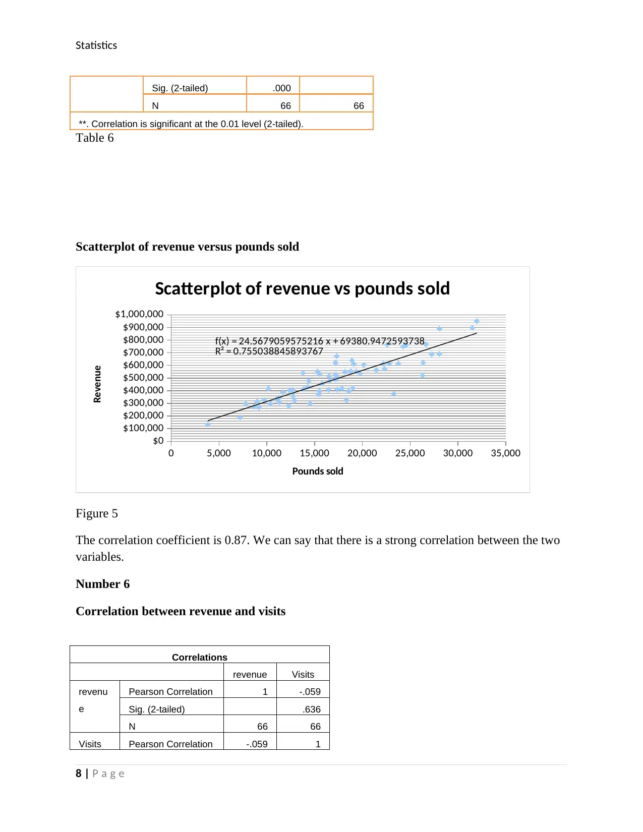
Number 5
Correlation of revenue and lbs sold
Correlations
revenue pounds_sold
revenue Pearson Correlation 1 .869**
Sig. (2-tailed) .000
N 66 66
pounds_sold Pearson Correlation .869** 1
7 | P a g e
Paraphrase This Document
Need a fresh take? Get an instant paraphrase of this document with our AI Paraphraser
Statistics
Sig. (2-tailed) .000
N 66 66
**. Correlation is significant at the 0.01 level (2-tailed).
Table 6
Scatterplot of revenue versus pounds sold
0 5,000 10,000 15,000 20,000 25,000 30,000 35,000
$0
$100,000
$200,000
$300,000
$400,000
$500,000
$600,000
$700,000
$800,000
$900,000
$1,000,000
f(x) = 24.5679059575216 x + 69380.9472593738
R² = 0.755038845893767
Scatterplot of revenue vs pounds sold
Pounds sold
Revenue
Figure 5
The correlation coefficient is 0.87. We can say that there is a strong correlation between the two
variables.
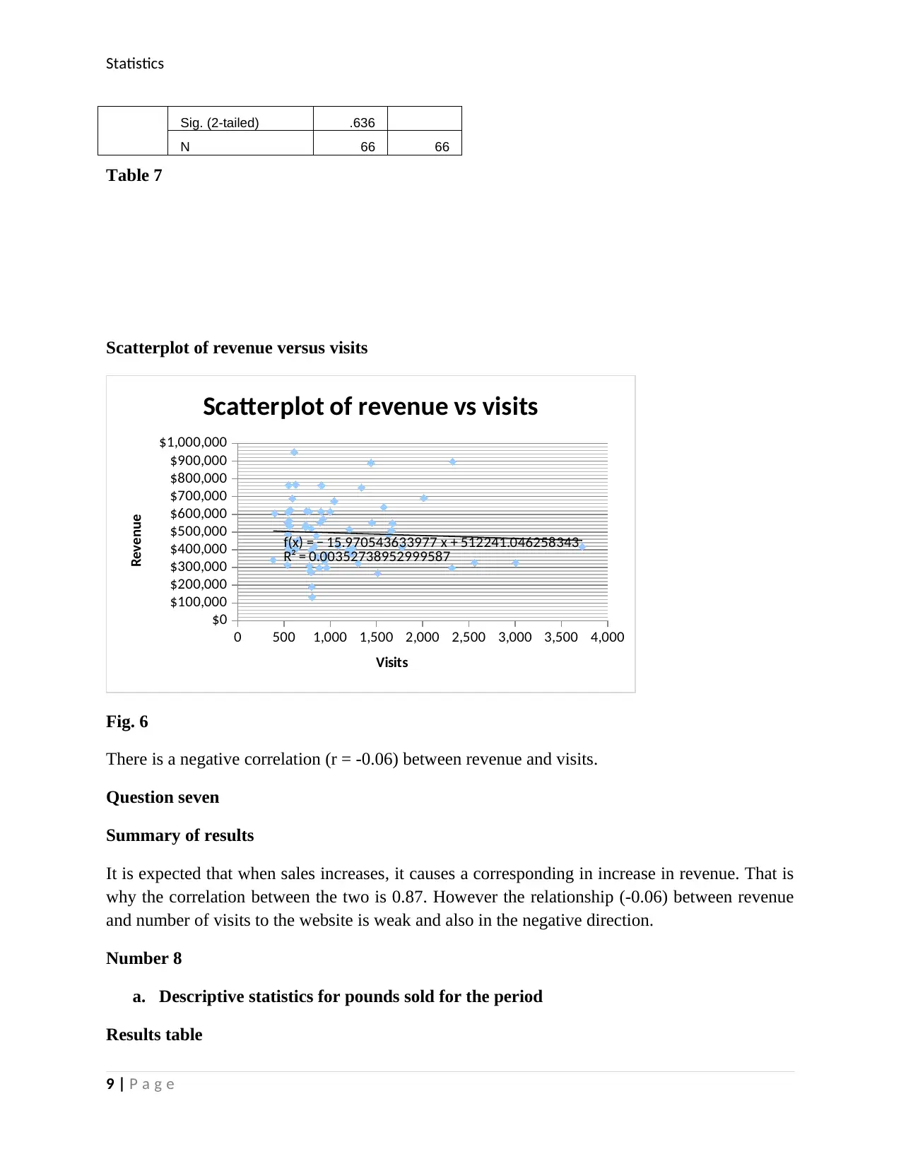
Number 6
Correlation between revenue and visits
Correlations
revenue Visits
revenu
e
Pearson Correlation 1 -.059
Sig. (2-tailed) .636
N 66 66
Visits Pearson Correlation -.059 1
8 | P a g e
Statistics
Sig. (2-tailed) .636
N 66 66
Table 7
Scatterplot of revenue versus visits
0 500 1,000 1,500 2,000 2,500 3,000 3,500 4,000
$0
$100,000
$200,000
$300,000
$400,000
$500,000
$600,000
$700,000
$800,000
$900,000
$1,000,000
f(x) = − 15.970543633977 x + 512241.046258343
R² = 0.00352738952999587
Scatterplot of revenue vs visits
Visits
Revenue
Fig. 6
There is a negative correlation (r = -0.06) between revenue and visits.
Question seven
Summary of results
It is expected that when sales increases, it causes a corresponding in increase in revenue. That is
why the correlation between the two is 0.87. However the relationship (-0.06) between revenue
and number of visits to the website is weak and also in the negative direction.
Number 8
a. Descriptive statistics for pounds sold for the period
Results table
9 | P a g e
Statistics
Lbs. Sold
Mean 18681.5551
7
Median 17673
Std Dev. 6840.50794
Min. 3826
Max. 44740
Table 8
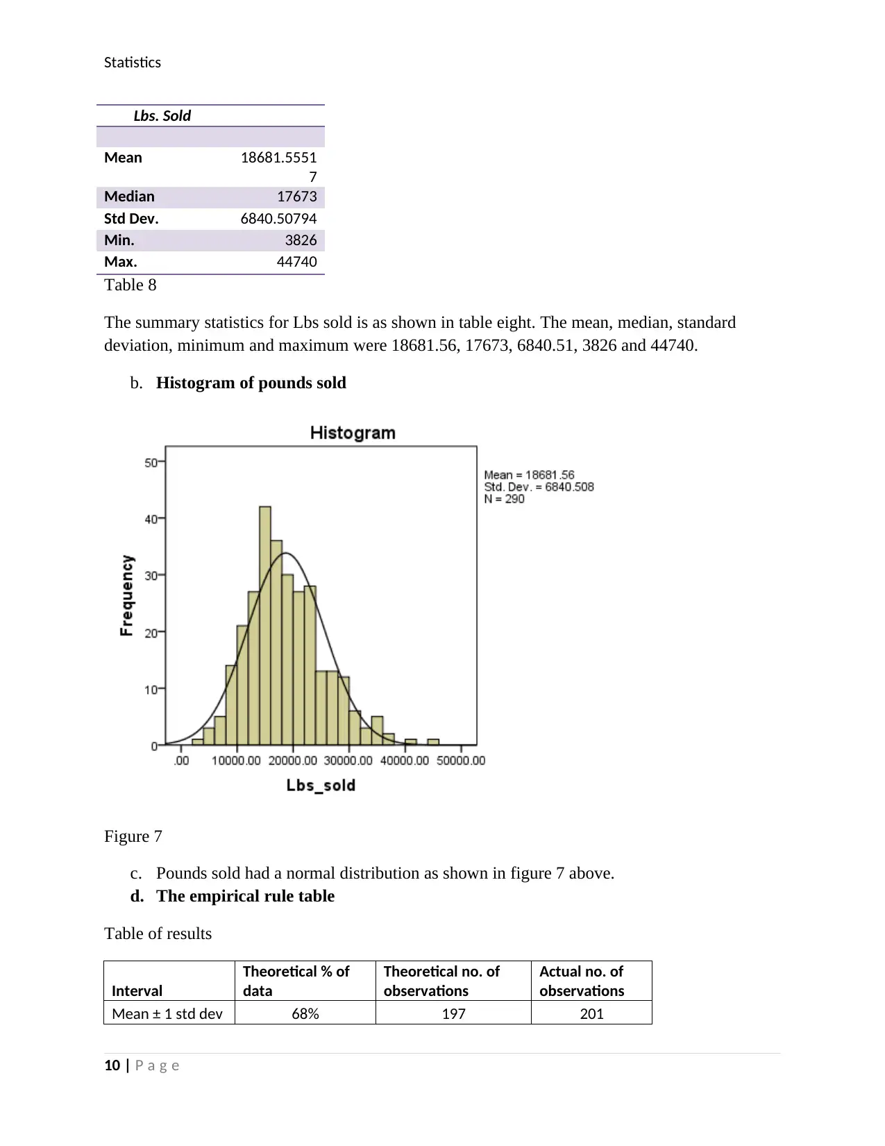
The summary statistics for Lbs sold is as shown in table eight. The mean, median, standard
deviation, minimum and maximum were 18681.56, 17673, 6840.51, 3826 and 44740.
b. Histogram of pounds sold
Figure 7
c. Pounds sold had a normal distribution as shown in figure 7 above.
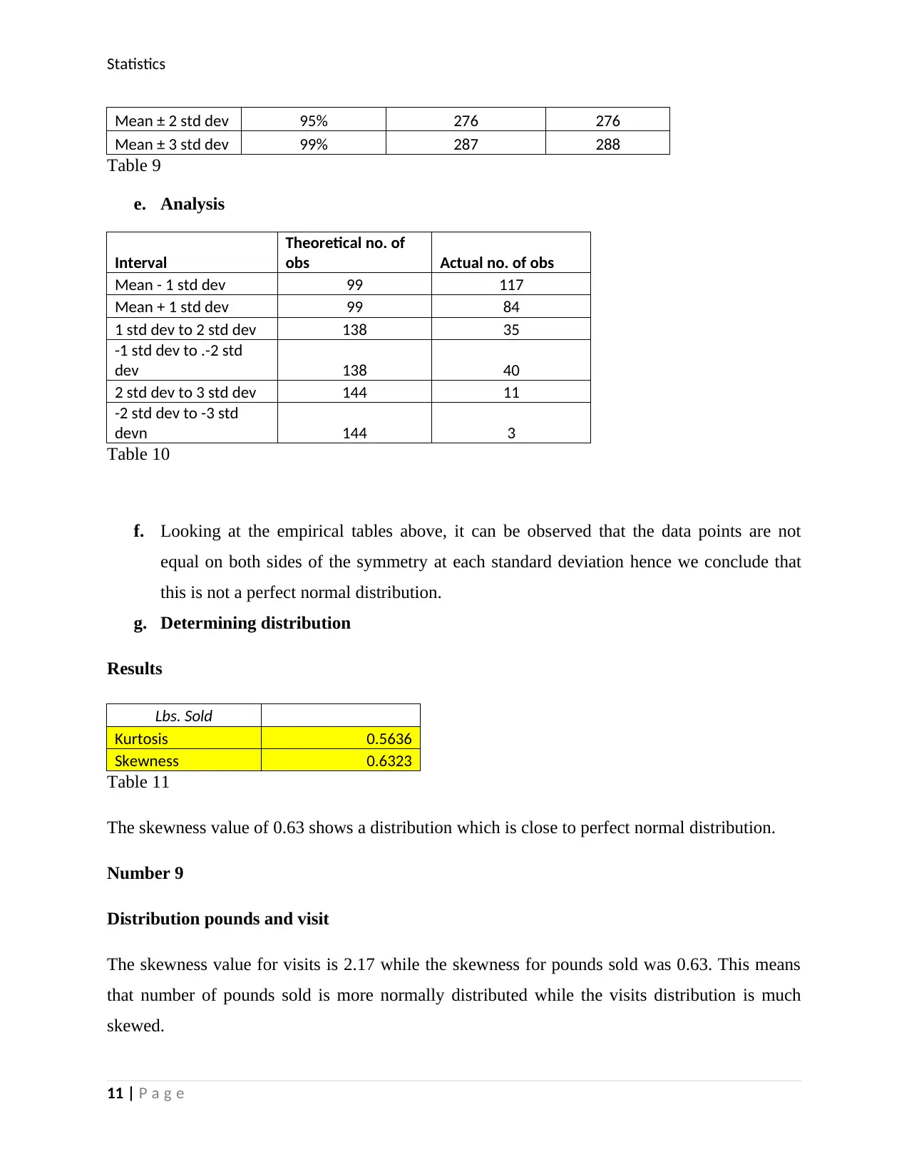
d. The empirical rule table
Table of results
Interval
Theoretical % of
data
Theoretical no. of
observations
Actual no. of
observations
Mean ± 1 std dev 68% 197 201
10 | P a g e
Secure Best Marks with AI Grader
Need help grading? Try our AI Grader for instant feedback on your assignments.
Statistics
Mean ± 2 std dev 95% 276 276
Mean ± 3 std dev 99% 287 288
Table 9
e. Analysis
Interval
Theoretical no. of
obs Actual no. of obs
Mean - 1 std dev 99 117
Mean + 1 std dev 99 84
1 std dev to 2 std dev 138 35
-1 std dev to .-2 std
dev 138 40
2 std dev to 3 std dev 144 11
-2 std dev to -3 std
devn 144 3
Table 10
f. Looking at the empirical tables above, it can be observed that the data points are not
equal on both sides of the symmetry at each standard deviation hence we conclude that
this is not a perfect normal distribution.
g. Determining distribution
Results
Lbs. Sold
Kurtosis 0.5636
Skewness 0.6323
Table 11
The skewness value of 0.63 shows a distribution which is close to perfect normal distribution.
Number 9
Distribution pounds and visit
The skewness value for visits is 2.17 while the skewness for pounds sold was 0.63. This means
that number of pounds sold is more normally distributed while the visits distribution is much
skewed.
11 | P a g e
Statistics
Number 10
Visits by traffic source bar chart
Referring Sites Search Engines Direct Traffic Other
0
5,000
10,000
15,000
20,000
25,000
30,000
35,000
40,000
45,000
38,754
20,964
9,709
4
Visits by traffic source
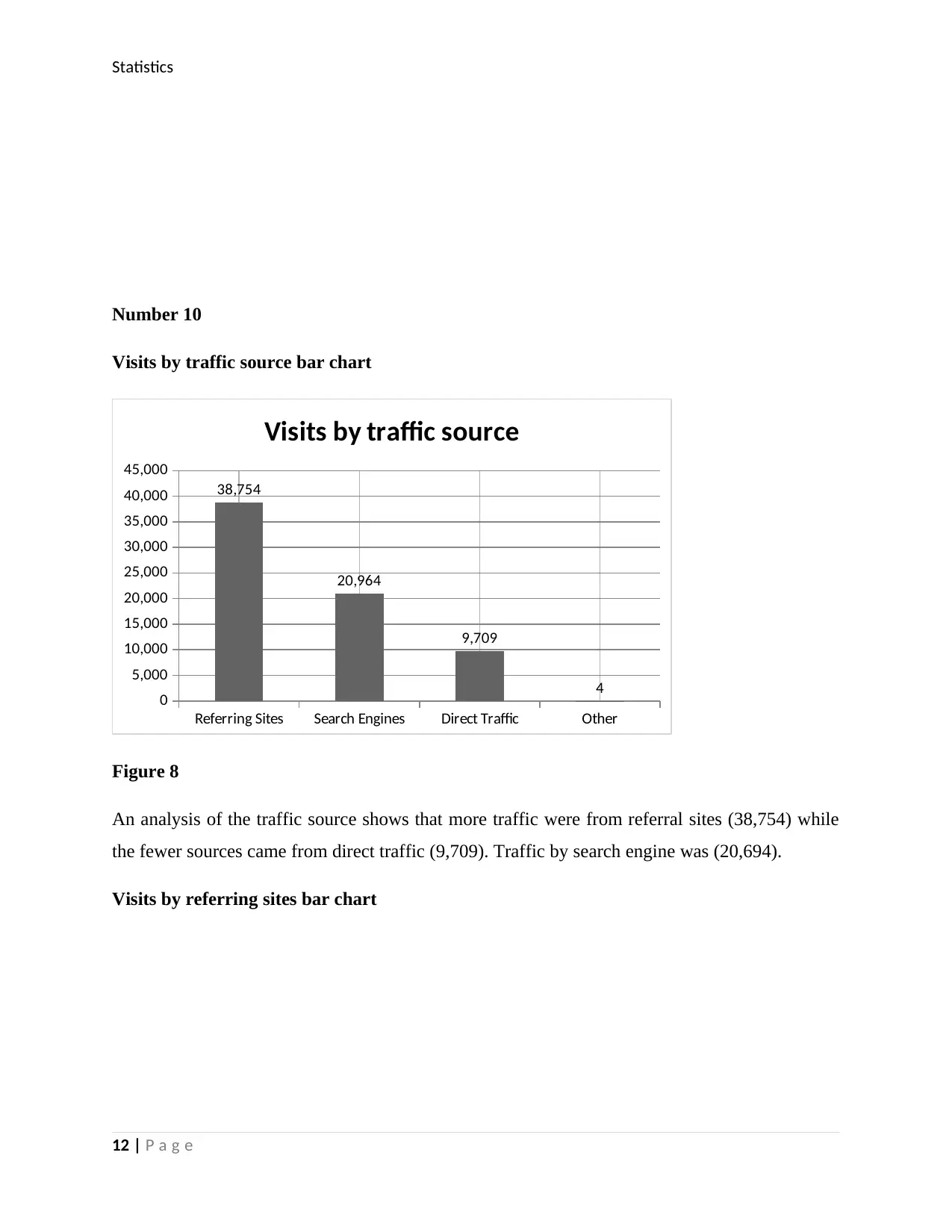
Figure 8
An analysis of the traffic source shows that more traffic were from referral sites (38,754) while
the fewer sources came from direct traffic (9,709). Traffic by search engine was (20,694).
Visits by referring sites bar chart
12 | P a g e
Statistics
googleads.g.doubleclick.net
pagead2.googlesyndication.com
sedoparking.com
globalspec.com
freepatentsonline.com
thomasnet.com
mu.com
mail.google.com
psicofxp.com
0
4,000
8,000
12,000
16,000 15,626
8,044
3,138
693 582 389 379 344 337 310
Visits by referring sites
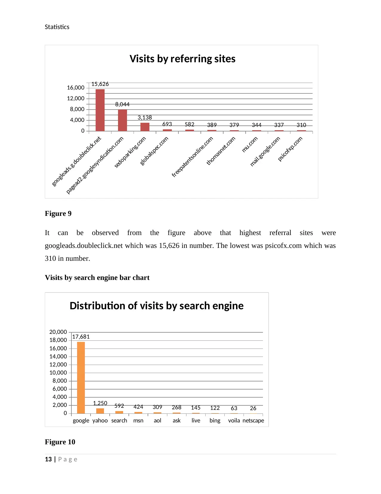
Figure 9
It can be observed from the figure above that highest referral sites were
googleads.doubleclick.net which was 15,626 in number. The lowest was psicofx.com which was
310 in number.
Visits by search engine bar chart
google yahoo search msn aol ask live bing voila netscape
0
2,000
4,000
6,000
8,000
10,000
12,000
14,000
16,000
18,000
20,000 17,681
1,250 592 424 309 268 145 122 63 26
Distribution of visits by search engine
Figure 10
13 | P a g e
Paraphrase This Document
Need a fresh take? Get an instant paraphrase of this document with our AI Paraphraser
Statistics
It can be observed from figure 10 that the highest used search engine was google which was
17,681in number. The lowest used search engine was netscape which was 26 in number.
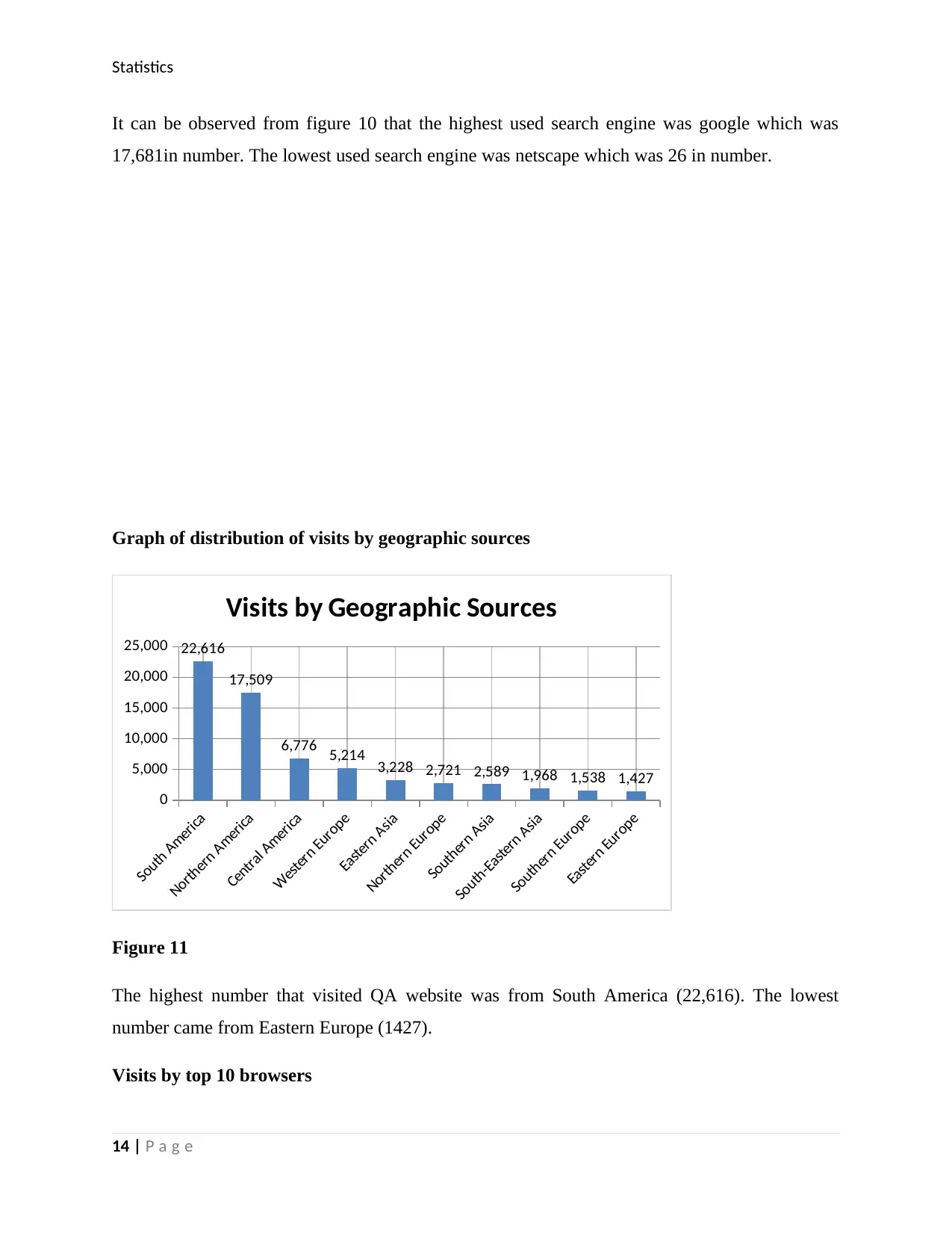
Graph of distribution of visits by geographic sources
South America
Northern America
Central America
Western Europe
Eastern Asia
Northern Europe
Southern Asia
South-Eastern Asia
Southern Europe
Eastern Europe
0
5,000
10,000
15,000
20,000
25,000 22,616
17,509
6,776 5,214 3,228 2,721 2,589 1,968 1,538 1,427
Visits by Geographic Sources
Figure 11
The highest number that visited QA website was from South America (22,616). The lowest
number came from Eastern Europe (1427).
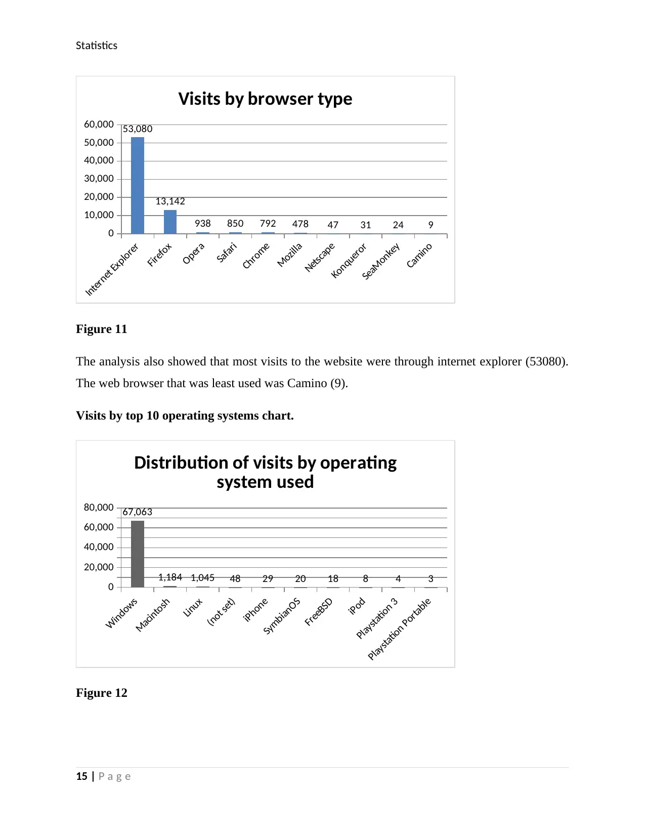
Visits by top 10 browsers
14 | P a g e
Statistics
Internet Explorer
Firefox
Opera
Safari
Chrome
Mozilla
Netscape
Konqueror
SeaMonkey
Camino
0
10,000
20,000
30,000
40,000
50,000
60,000 53,080
13,142
938 850 792 478 47 31 24 9
Visits by browser type
Figure 11
The analysis also showed that most visits to the website were through internet explorer (53080).
The web browser that was least used was Camino (9).
Visits by top 10 operating systems chart.
Windows
Macintosh
Linux
(not set)
iPhone
SymbianOS
FreeBSD
iPod
Playstation 3
Playstation Portable
0
20,000
40,000
60,000
80,000 67,063
1,184 1,045 48 29 20 18 8 4 3
Distribution of visits by operating
system used
Figure 12
15 | P a g e

Statistics
The operating systems that were used to access the website were also analyzed. As can be seen
from figure 12, the most used was windows which was 67,063 while the least used was
playstation portable which was 3 in number.
16 | P a g e
The operating systems that were used to access the website were also analyzed. As can be seen
from figure 12, the most used was windows which was 67,063 while the least used was
playstation portable which was 3 in number.
16 | P a g e
1 out of 16
Related Documents
Your All-in-One AI-Powered Toolkit for Academic Success.
+13062052269
info@desklib.com
Available 24*7 on WhatsApp / Email
![[object Object]](/_next/static/media/star-bottom.7253800d.svg)
Unlock your academic potential
© 2024 | Zucol Services PVT LTD | All rights reserved.


