Stock Return Analysis

This document provides an analysis of stock returns, including hypothesis testing of means, variances, and homoskedasticity. It also covers regression analysis and inference in stock analysis.

Stock Analysis 1
STOCK RETURN ANALYSIS
by[Name]
Course
Professor’s Name
Institution
Location of Institution
Date

Stock Analysis 2
Stock Return Analysis
Task A: Downloading the Dataset
The data was obtained from the links provided by the lecturer.
Task B: Hypothesis Testing of Means and Variance equality
1. Returns Computation and Normality test
Jarque-Berra test of normality is based on the following hypothesis:
H0: X N (μ, σ 2); The series is normally distributed (Das and Imon 2016)
H1: The series is not normally distributed.
The test statics is given as:
JB= n
6 ( S2 + K2
4 )
Where:
S – the sample skewness
K- sample excess kurtosis (excess kurtosis minus 3)
n – the number of non-missing values in the data sample
The JB statistic has an asymptotic Chi-square distribution with two degrees of
freedom under the null hypothesis
JB χ v=2 ,α
2 v – is the degrees of freedom and α – significance level.
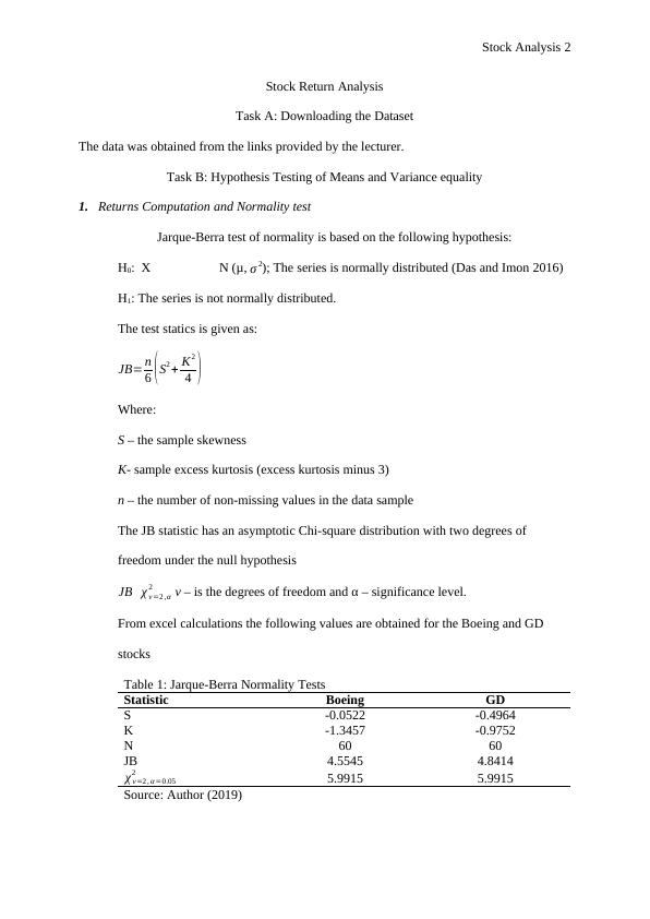
From excel calculations the following values are obtained for the Boeing and GD
stocks
Table 1: Jarque-Berra Normality Tests
Statistic Boeing GD
S -0.0522 -0.4964
K -1.3457 -0.9752
N 60 60
JB 4.5545 4.8414
χ v=2 , α =0.05
2
5.9915 5.9915
Source: Author (2019)

Stock Analysis 3
The calculated JB for Boeing return is 4.5545 less than 5.9915 implying that at
95% level of significance the Boeing return sampling distribution is normally
distributed. Similarly, the calculated JB for GD return is 4.8414 less than 5.9915
implying that at 95% level of significance the GD return sampling distribution is
normally distributed.
2. Hypothesis testing of a single population mean (μ)
The hypothesis testing takes the following steps.
Hypothesis under test:
Ho: μ = 2.8% against H1: μ ≠ 2.8%
Significance level = 0.05.
Test statistic: One sample t-tests given as
tcalc .= √n ( X−μ0 )
SD
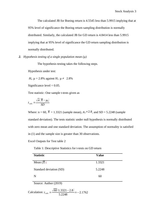
Where: n = 60, X = 1.3321 (sample mean), μ0 =2.8, and SD = 5.2248 (sample
standard deviation). The tests statistic under null hypothesis is normally distributed
with zero mean and one standard deviation. The assumption of normality is satisfied
in (1) and the sample size is greater than 30 observations.
Excel Outputs for Test table 2
Table 1: Descriptive Statistics for t-tests on GD return
Statistic Value
Mean ( X ¿ 1.3321
Standard deviation (SD) 5.2248
N 60
Source: Author (2019)
Calculation: tcalc .= √60 ( 1.3321−2.8 )
5.2248 =−2.1762

Stock Analysis 4
Decision Criteria: Reject null hypothesis if |tcalc .| ≥ ttab. Where ttab = t α
2 ,59=2.300
Decision: Since |tcalc .| = 2.1762 < ttab = 2.300 fail to reject null hypothesis and
conclude that at 95% level of significance we have sufficient evidence that the
average return on GD stock is not different from 2.8%. Therefore, on average the
return on GD stock will be 2.8%.
3. Hypothesis testing of homoskedasticity
The test is Bartlett’s test based on the following hypothesis:
Ho: Existence of homoskedasticity (The risk associated with Boeing stock is similar to
that associated with GD stock)
H1: Heteroskedasticity (The risk associated with Boeing stock is different to that
associated with GD stock)
Significance level = 0.05
Test statistic: Bartlett’s statistic (computed in excel).
B=
( n−k ) ln ( S2 )−∑
j=1
k
( n j−1 ) ln S j
2
c
Where: S2 is the pooled variance, n -sample size, k-number of stocks, and
c=1+ 1
3 ( k −1 ) (∑
j=1
k 1
n j−1 − 1
n−k )
Under the null hypothesis B χ ( k−1 )
2 (Hosken, Buss and Hodgson 2018).
From excel B = 0.0000 and B-critical = 3.841. Decision reject fail to reject null
hypothesis and conclude that at 95% level of significance there is sufficient evidence
to support that the risk associated with Boeing stock is similar to that associated with
GD stock.
4. Hypothesis testing of two population means

Stock Analysis 5
The population variances are unknown then we use two independent t-tests with the
following steps:
Parameter = μ1 - μ2, the difference between the population average return of Boeing
stock, μ1, and the difference between the population average return of GD stock, μ2.
Hypothesis
Ho: μ1 - μ2 = 0, there is no difference in the population average stock return
H1: μ1 - μ2 ≠ 0, there is a difference in the population average stock return
Significance level = 0.05
Test statistic: 95% confidence interval. The results of the analysis are presented in
table 3.
Table 3: t-Test: Two-Sample Assuming Equal Variances
Statistic Boeing Stock GD Stock
Mean 1.8923 1.3321
Variance 42.5361 27.2981
Observations 60 60
Pooled Variance 34.9171
t Critical two-tail 1.9803
Source: Author (2019)
The 95% CI is calculated as follows:
( X1−X2 ) ± t∗Pooled variance∗ √ 2
n
X1 −X2=1.8923−1.3321=0.5602
0.5602 ±1.9803∗34.9171∗
√ 2
60
0.5602 ±12.6243
Then, 95% CI is (-12.0641, 13.1845).

Stock Analysis 6
Decision: Since the CI contains zero, we fail to reject the null hypothesis and conclude that at
95 level of significance, there is sufficient evidence to conclude that the population average
for both stocks are the same. Given this information I would prefer, the GD stock because it
has the lowest variance implying lowest standard deviation. Therefore, the return on GD
stock is relatively stable.
Task C: Regression Analysis and Inference
5. Regression analysis
(a) The market is the return on S&P500 index and the response variable is excess
market return on GD stock return. The explanatory variable is excess market
return (Xt). The regression output is presented in table 4.
Table 4: Regression Output
Coefficient SE t-value P-value
Lower
(95%)
Upper
(95%)
Intercept 0.613 0.57353 1.06957 0.28925 -0.53462 1.761478
Xt 0.986 0.07113 13.85970 0.00000 0.84346 1.128225
F 192.0914 P-value(F) <0.000
R-squared 0.768085
Source: Author (2019)
The estimated CAPM model is Yt = 0.613 + 0.986Xt.
(b) The Bi is greater than 0 implying that the asset is exposed to market risk and Rt is
greater than rf provided that E[Rm,t – rf] >0.
(c) The R2 = 0.7681 indicating that 76.81% of changes in the excess market return on
GD stock are as a result of changes in the excess market return.

Stock Analysis 7
(d) The 95% CI is (0.8435, 1.1282) implying that the true sensitivity to the market
risk for the excess market return lies between 0.8435 and 1.1282.
6. The hypothesis to test
H0: B = 1 (The GD stock is aggressive)
H1: B = 0 (the GD stock is not aggressive)
Significance level = 0.05
Test statistic: B/SE = 0.986/0.07113 = 13.86.
Since the ratio is greater than one the GD stock is aggressive.
7. The verification of normality assumption involves two steps. The first step is the
graphical examination. The figure 1 below shows the normality plot of the residuals.
0 20 40 60 80 100 120
-30
-20
-10
0
10
20
30
Figure 1: Normal Probability Plot
Sample Percentile
Yt
The plots show majority of the points on or close to the diagonal line and indication that
the residuals might be normally distributed. However, to confirm the observation, Jarque-
Berra test of normality is used. The test is based on the following hypothesis:
H0: X N (μ, σ 2); The residuals are normally distributed
H1: The residuals are not normally distributed.
The Jarque-Berra test performed in excel produced the following results JB = 2.8125
while the Test value is 5.999. Therefore, we fail to reject the null hypothesis that the
residuals are normally distributed. Hence, the assumption of normality is valid. T\

Stock Analysis 8
References
Das, K.R. and Imon, A.H.M.R., 2016. A brief review of tests for normality. American
Journal of Theoretical and Applied Statistics, 5(1), pp.5-12.
Hosken, D.J., Buss, D.L. and Hodgson, D.J., 2018. Beware the F test (or, how to compare
variances). Animal Behaviour, 136, pp.119-126.