Rotary Inverted Pendulum Analysis and Controller Design Project
VerifiedAdded on 2023/04/21
|22
|3372
|79
Project
AI Summary
This project report details the design and analysis of a Rotary Inverted Pendulum system. The student begins by introducing the concept and objectives, followed by a step-by-step guide to building an inverted pendulum model in Simulink. The report then explores open-loop impulse responses, system poles and zeros, and the process of linearization. The core of the project focuses on controller design using the pole placement method, including full-state feedback and the use of MATLAB functions. The report also includes analysis of the closed-loop system's response, utilizing the Control System Designer in MATLAB, and concludes with a discussion of the inverted pendulum's behavior and analytical and physical modeling approaches, supported by figures and MATLAB code snippets.

University
*** Semester
Inverted Pendulum
Student Name:
Register Number:
Submission Date:
*** Semester
Inverted Pendulum
Student Name:
Register Number:
Submission Date:
Paraphrase This Document
Need a fresh take? Get an instant paraphrase of this document with our AI Paraphraser

Table of Contents
1. Introduction............................................................................................................................................................ 1
Question-1.................................................................................................................................................................... 1
Question-2.................................................................................................................................................................... 1
Question-3.................................................................................................................................................................... 3
Question-4.................................................................................................................................................................... 3
Question-5.................................................................................................................................................................... 6
Question-6.................................................................................................................................................................... 6
Question-7.................................................................................................................................................................... 8
Question-8.................................................................................................................................................................. 11
Question-9.................................................................................................................................................................. 12
2. Conclusion............................................................................................................................................................. 14
References...................................................................................................................................................................... 15
1. Introduction
The Rotary Servo Base Unit is attached with a Rotary Inverted Pendulum (RIP) module,
which expands mechatronics along with the controls topics which could be instructed. It is a
known fact that the pendulum module is challenging for the students for modelling and
controlling the pendulum. However, it is also challenging to learn the hybrid control systems by
means of tuning the swing-up control systems. Additionally, along with teaching the concepts of
intermediate control, the Rotary Inverted Pendulum could be used for the research in various
fields, involving the fluffy control.
Question-1
ANSWER:
Introduction
The Rotary Inverted Pendulum is an exemplary control issue that is investigated
frequently as an undertaking in control courses because of its effectively created elements that
are a mix of its multifaceted nature of control design. It is a system which is built using the
pendulum that is attached to the rotary arm’s end, which the motor controls. In general, the motor
includes the servomotor coupled, by using the gear-chain. The principle objective includes
keeping the pendulum in the upright position of unsteady equilibrium. The next objective
includes keeping the motor at the specifically mentioned angular position, when the first task is
being performed (Gao & Li, 2011). Whereas, the last task includes destabilizing the motor
starting from the hanging position of the equilibrium which is not stable, with the goal to achieve
the stability range (i.e., here the mode controller could easily start the stabilization.)
Aim
The aim includes designing the controller for the ROTPEN kit, with the help of an
effective linearised pendulum model.
Question-2
1
⊘ This is a preview!⊘
Do you want full access?
Subscribe today to unlock all pages.
Trusted by 1+ million students worldwide
ANSWER:
The below mentioned steps help to build the inverted pendulum model in Simulink, they
are,
1) In the MATLAB command window type Simulink and it opens the Simulink
environment. Next, in Simulink open a new model window by selecting New >
Simulink > Blank Model of the open Simulink Start Page window or by
pressing Ctrl-N.
2) From the Simulink/User-Defined Functions library, 4 Fcn Blocks are inserted. The
following equations for , , , and are built by employing the blocks.
3) Every single Fcn block must be changed so that it matches with its linked function.
4) From the Simulink/Continuous library4 Integrator blocks must be inserted. Every
single Integrator block’s output will be the system’s state variable, , , , and .
5) Every single Integrator block must be double-clicked for adding the “State Name:” of
the linked state variable. Next, the “Initial condition:” must be changed for
(pendulum angle) to "pi", for representing that the pendulum starts to point straight up.
6) From the Simulink/Signal Routing library, 4 Multiplexer (Mux) blocks must be
inserted, for every single Fcn block.
7) From the Simulink/Sinks and Simulink/Sources libraries, 2 Out1 blocks and one In1
block must be inserted, respectively. Next, the labels must be double-clicked, as it
helps to change the names of the blocks. For "Position" of the cart and the "Angle" of
the pendulum, two outputs are provided when one input is for "Force" that is applied
on the cart.
8) Mux blocks’ each output is connected to the corresponding input of the Fcn block.
9) In the function blocks the below equations are filled (Zulkarnain Shaharudin & Abdul
Rashid Husain., 2013).
( J eq+ M p r2 ) ¨θ + M p Lp rsinα ( ˙α )2−M p Lp rcosα ¨α=τ output−β1 ˙θ
4
3 M p Lp
2 ¨α −M p Lp rcosα ¨θ−Mp g Lp sinα=− β2 ˙α
τ output= Kt [ V m−Km ˙θ (t) ]
Rm
2
Paraphrase This Document
Need a fresh take? Get an instant paraphrase of this document with our AI Paraphraser
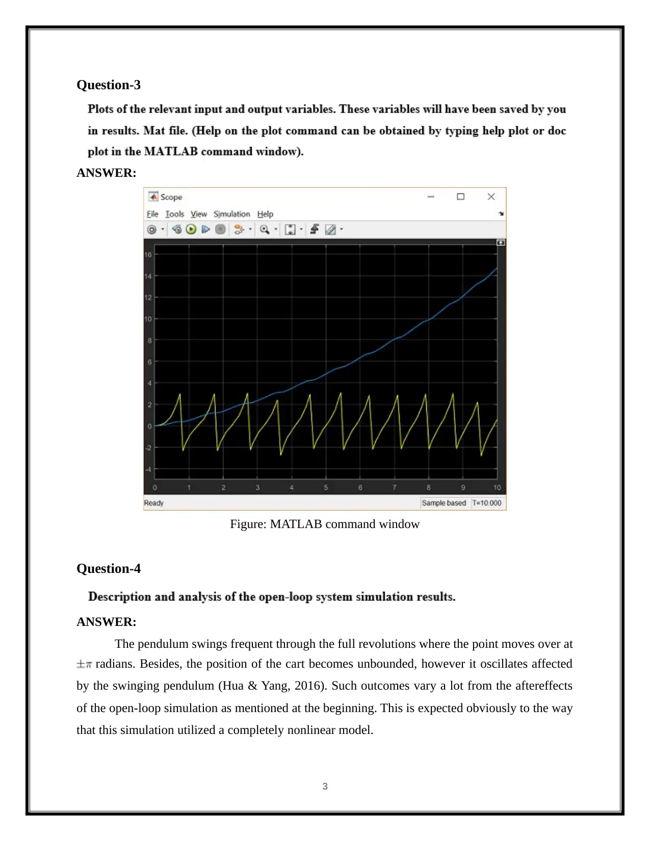
Question-3
ANSWER:
Figure: MATLAB command window
Question-4
ANSWER:
The pendulum swings frequent through the full revolutions where the point moves over at
radians. Besides, the position of the cart becomes unbounded, however it oscillates affected
by the swinging pendulum (Hua & Yang, 2016). Such outcomes vary a lot from the aftereffects
of the open-loop simulation as mentioned at the beginning. This is expected obviously to the way
that this simulation utilized a completely nonlinear model.
3
ANSWER:
Figure: MATLAB command window
Question-4
ANSWER:
The pendulum swings frequent through the full revolutions where the point moves over at
radians. Besides, the position of the cart becomes unbounded, however it oscillates affected
by the swinging pendulum (Hua & Yang, 2016). Such outcomes vary a lot from the aftereffects
of the open-loop simulation as mentioned at the beginning. This is expected obviously to the way
that this simulation utilized a completely nonlinear model.
3
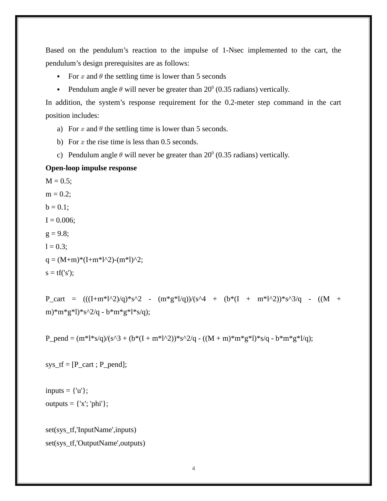
Based on the pendulum’s reaction to the impulse of 1-Nsec implemented to the cart, the
pendulum’s design prerequisites are as follows:
For and the settling time is lower than 5 seconds
Pendulum angle will never be greater than 200 (0.35 radians) vertically.
In addition, the system’s response requirement for the 0.2-meter step command in the cart
position includes:
a) For and the settling time is lower than 5 seconds.
b) For the rise time is less than 0.5 seconds.
c) Pendulum angle will never be greater than 200 (0.35 radians) vertically.
Open-loop impulse response
M = 0.5;
m = 0.2;
b = 0.1;
I = 0.006;
g = 9.8;
l = 0.3;
q = (M+m)*(I+m*l^2)-(m*l)^2;
s = tf('s');
P_cart = (((I+m*l^2)/q)*s^2 - (m*g*l/q))/(s^4 + (b*(I + m*l^2))*s^3/q - ((M +
m)*m*g*l)*s^2/q - b*m*g*l*s/q);
P_pend = (m*l*s/q)/(s^3 + (b*(I + m*l^2))*s^2/q - ((M + m)*m*g*l)*s/q - b*m*g*l/q);
sys_tf = [P_cart ; P_pend];
inputs = {'u'};
outputs = {'x'; 'phi'};
set(sys_tf,'InputName',inputs)
set(sys_tf,'OutputName',outputs)
4
⊘ This is a preview!⊘
Do you want full access?
Subscribe today to unlock all pages.
Trusted by 1+ million students worldwide
t=0:0.01:1;
impulse(sys_tf,t);
title('Open-Loop Impulse Response')
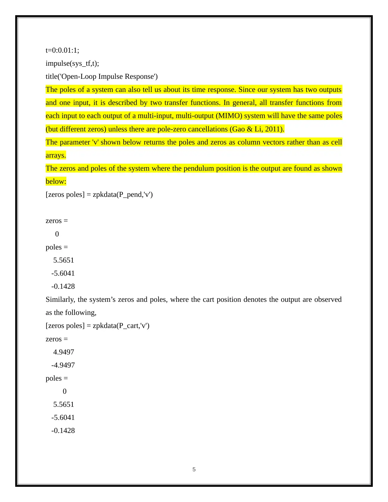
The poles of a system can also tell us about its time response. Since our system has two outputs
and one input, it is described by two transfer functions. In general, all transfer functions from
each input to each output of a multi-input, multi-output (MIMO) system will have the same poles
(but different zeros) unless there are pole-zero cancellations (Gao & Li, 2011).
The parameter 'v' shown below returns the poles and zeros as column vectors rather than as cell
arrays.
The zeros and poles of the system where the pendulum position is the output are found as shown
below:
[zeros poles] = zpkdata(P_pend,'v')
zeros =
0
poles =
5.5651
-5.6041
-0.1428
Similarly, the system’s zeros and poles, where the cart position denotes the output are observed
as the following,
[zeros poles] = zpkdata(P_cart,'v')
zeros =
4.9497
-4.9497
poles =
0
5.5651
-5.6041
-0.1428
5
impulse(sys_tf,t);
title('Open-Loop Impulse Response')
The poles of a system can also tell us about its time response. Since our system has two outputs
and one input, it is described by two transfer functions. In general, all transfer functions from
each input to each output of a multi-input, multi-output (MIMO) system will have the same poles
(but different zeros) unless there are pole-zero cancellations (Gao & Li, 2011).
The parameter 'v' shown below returns the poles and zeros as column vectors rather than as cell
arrays.
The zeros and poles of the system where the pendulum position is the output are found as shown
below:
[zeros poles] = zpkdata(P_pend,'v')
zeros =
0
poles =
5.5651
-5.6041
-0.1428
Similarly, the system’s zeros and poles, where the cart position denotes the output are observed
as the following,
[zeros poles] = zpkdata(P_cart,'v')
zeros =
4.9497
-4.9497
poles =
0
5.5651
-5.6041
-0.1428
5
Paraphrase This Document
Need a fresh take? Get an instant paraphrase of this document with our AI Paraphraser
Question-5
ANSWER:
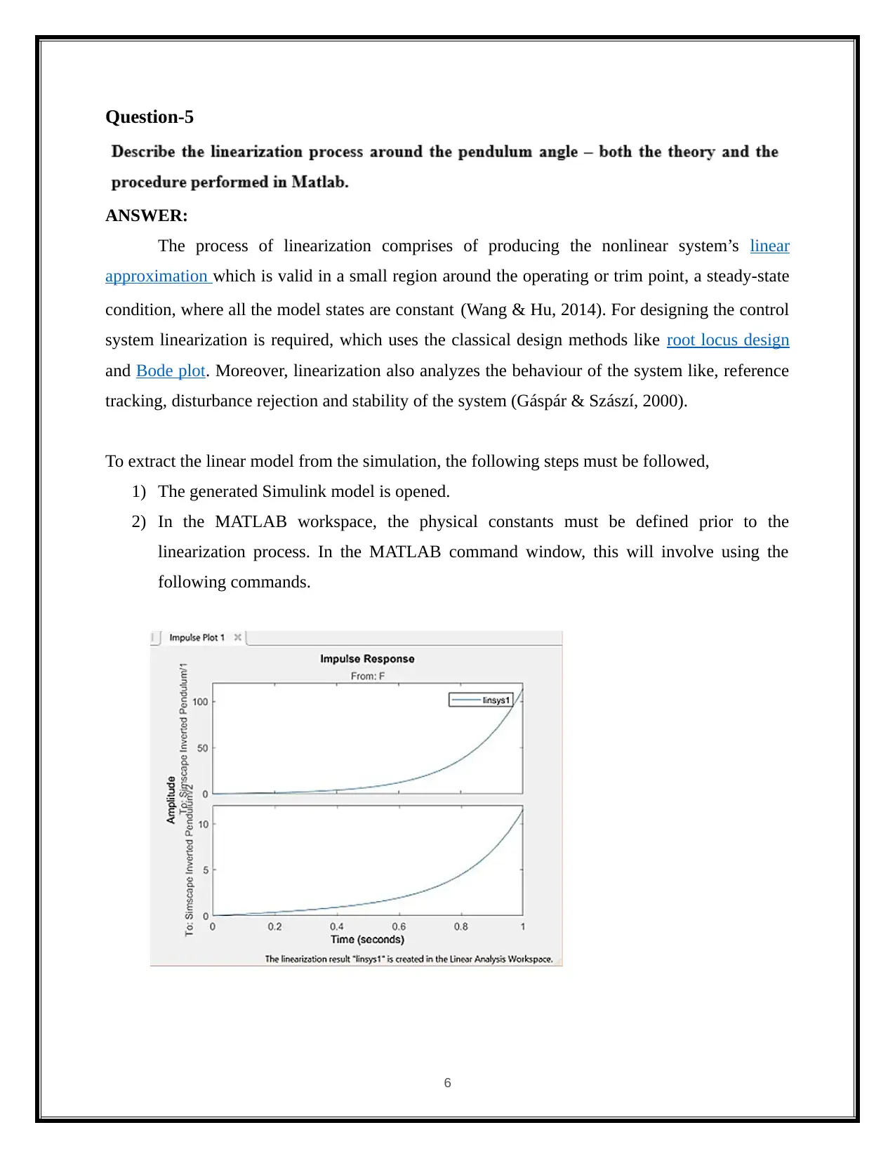
The process of linearization comprises of producing the nonlinear system’s linear
approximation which is valid in a small region around the operating or trim point, a steady-state
condition, where all the model states are constant (Wang & Hu, 2014). For designing the control
system linearization is required, which uses the classical design methods like root locus design
and Bode plot. Moreover, linearization also analyzes the behaviour of the system like, reference
tracking, disturbance rejection and stability of the system (Gáspár & Szászí, 2000).
To extract the linear model from the simulation, the following steps must be followed,
1) The generated Simulink model is opened.
2) In the MATLAB workspace, the physical constants must be defined prior to the
linearization process. In the MATLAB command window, this will involve using the
following commands.
6
ANSWER:
The process of linearization comprises of producing the nonlinear system’s linear
approximation which is valid in a small region around the operating or trim point, a steady-state
condition, where all the model states are constant (Wang & Hu, 2014). For designing the control
system linearization is required, which uses the classical design methods like root locus design
and Bode plot. Moreover, linearization also analyzes the behaviour of the system like, reference
tracking, disturbance rejection and stability of the system (Gáspár & Szászí, 2000).
To extract the linear model from the simulation, the following steps must be followed,
1) The generated Simulink model is opened.
2) In the MATLAB workspace, the physical constants must be defined prior to the
linearization process. In the MATLAB command window, this will involve using the
following commands.
6
Question-6
ANSWER:
The pole placement method is utilized for building the controller of this system. To
measure the position of the pendulum, to measure the velocity of the pendulum and to measure
the pendulum displacement, this system needs a sensor (Angeli, 2001).
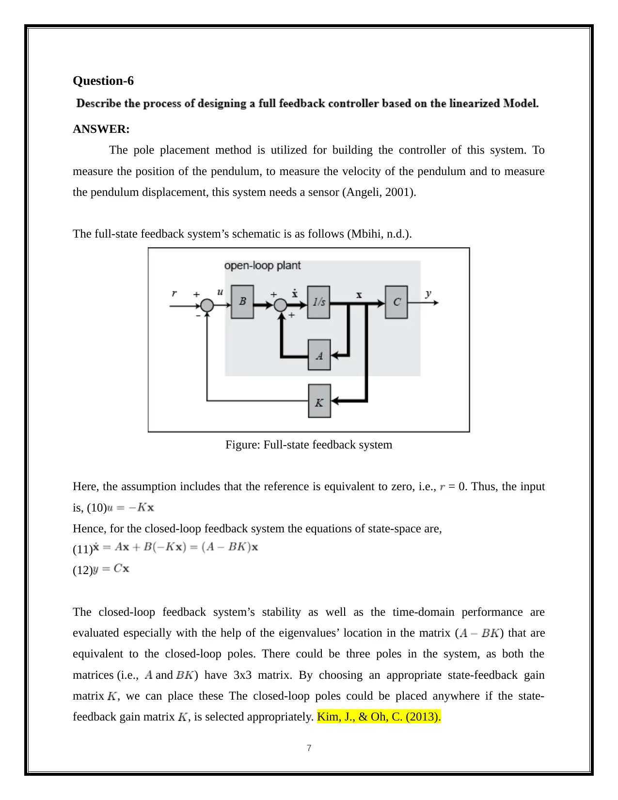
The full-state feedback system’s schematic is as follows (Mbihi, n.d.).
Figure: Full-state feedback system
Here, the assumption includes that the reference is equivalent to zero, i.e., = 0. Thus, the input
is, (10)
Hence, for the closed-loop feedback system the equations of state-space are,
(11)
(12)
The closed-loop feedback system’s stability as well as the time-domain performance are
evaluated especially with the help of the eigenvalues’ location in the matrix ( ) that are
equivalent to the closed-loop poles. There could be three poles in the system, as both the
matrices (i.e., and ) have 3x3 matrix. By choosing an appropriate state-feedback gain
matrix , we can place these The closed-loop poles could be placed anywhere if the state-
feedback gain matrix , is selected appropriately. Kim, J., & Oh, C. (2013).
7
ANSWER:
The pole placement method is utilized for building the controller of this system. To
measure the position of the pendulum, to measure the velocity of the pendulum and to measure
the pendulum displacement, this system needs a sensor (Angeli, 2001).
The full-state feedback system’s schematic is as follows (Mbihi, n.d.).
Figure: Full-state feedback system
Here, the assumption includes that the reference is equivalent to zero, i.e., = 0. Thus, the input
is, (10)
Hence, for the closed-loop feedback system the equations of state-space are,
(11)
(12)
The closed-loop feedback system’s stability as well as the time-domain performance are
evaluated especially with the help of the eigenvalues’ location in the matrix ( ) that are
equivalent to the closed-loop poles. There could be three poles in the system, as both the
matrices (i.e., and ) have 3x3 matrix. By choosing an appropriate state-feedback gain
matrix , we can place these The closed-loop poles could be placed anywhere if the state-
feedback gain matrix , is selected appropriately. Kim, J., & Oh, C. (2013).
7
⊘ This is a preview!⊘
Do you want full access?
Subscribe today to unlock all pages.
Trusted by 1+ million students worldwide
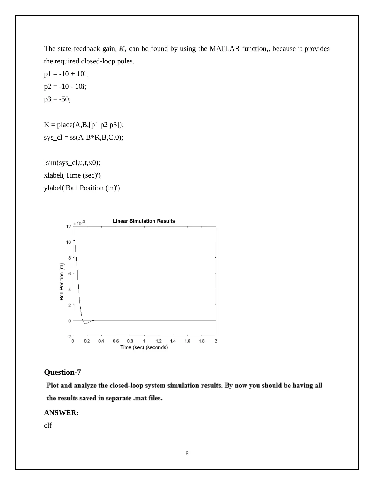
The state-feedback gain, , can be found by using the MATLAB function,, because it provides
the required closed-loop poles.
p1 = -10 + 10i;
p2 = -10 - 10i;
p3 = -50;
K = place(A,B,[p1 p2 p3]);
sys_cl = ss(A-B*K,B,C,0);
lsim(sys_cl,u,t,x0);
xlabel('Time (sec)')
ylabel('Ball Position (m)')
Question-7
ANSWER:
clf
8
the required closed-loop poles.
p1 = -10 + 10i;
p2 = -10 - 10i;
p3 = -50;
K = place(A,B,[p1 p2 p3]);
sys_cl = ss(A-B*K,B,C,0);
lsim(sys_cl,u,t,x0);
xlabel('Time (sec)')
ylabel('Ball Position (m)')
Question-7
ANSWER:
clf
8
Paraphrase This Document
Need a fresh take? Get an instant paraphrase of this document with our AI Paraphraser
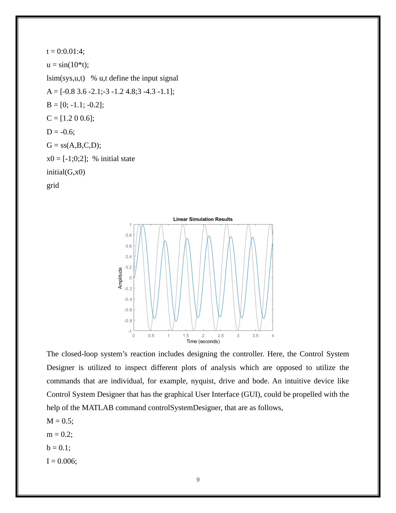
t = 0:0.01:4;
u = sin(10*t);
lsim(sys,u,t) % u,t define the input signal
A = [-0.8 3.6 -2.1;-3 -1.2 4.8;3 -4.3 -1.1];
B = [0; -1.1; -0.2];
C = [1.2 0 0.6];
D = -0.6;
G = ss(A,B,C,D);
x0 = [-1;0;2]; % initial state
initial(G,x0)
grid
The closed-loop system’s reaction includes designing the controller. Here, the Control System
Designer is utilized to inspect different plots of analysis which are opposed to utilize the
commands that are individual, for example, nyquist, drive and bode. An intuitive device like
Control System Designer that has the graphical User Interface (GUI), could be propelled with the
help of the MATLAB command controlSystemDesigner, that are as follows,
M = 0.5;
m = 0.2;
b = 0.1;
I = 0.006;
9

g = 9.8;
l = 0.3;
q = (M+m)*(I+m*l^2)-(m*l)^2;
s = tf('s');
P_pend = (m*l*s/q)/(s^3 + (b*(I + m*l^2))*s^2/q - ((M + m)*m*g*l)*s/q - b*m*g*l/q);
[zeros poles] = zpkdata(P_pend,'v')
zeros =
0
poles =
5.5651
-5.6041
-0.1428
controlSystemDesigner('bode',P_pend)
10
l = 0.3;
q = (M+m)*(I+m*l^2)-(m*l)^2;
s = tf('s');
P_pend = (m*l*s/q)/(s^3 + (b*(I + m*l^2))*s^2/q - ((M + m)*m*g*l)*s/q - b*m*g*l/q);
[zeros poles] = zpkdata(P_pend,'v')
zeros =
0
poles =
5.5651
-5.6041
-0.1428
controlSystemDesigner('bode',P_pend)
10
⊘ This is a preview!⊘
Do you want full access?
Subscribe today to unlock all pages.
Trusted by 1+ million students worldwide
1 out of 22
Related Documents


Your All-in-One AI-Powered Toolkit for Academic Success.
+13062052269
info@desklib.com
Available 24*7 on WhatsApp / Email
![[object Object]](/_next/static/media/star-bottom.7253800d.svg)
Unlock your academic potential
Copyright © 2020–2026 A2Z Services. All Rights Reserved. Developed and managed by ZUCOL.