Rotary Inverted Pendulum Report 2019 - System Modeling and Control

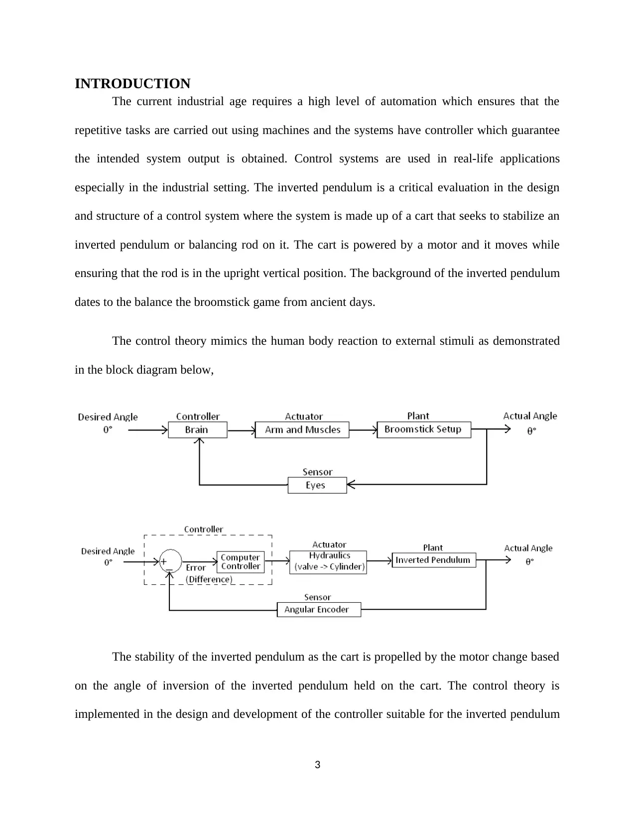
This report provides a comprehensive analysis of a rotary inverted pendulum system, covering system modeling, controller design, simulation, and experimental aspects. It begins with an introduction to the inverted pendulum concept and its real-world applications, followed by a detailed explanation of system modeling using Euler and Lagrangian methods. The report discusses controller design, including linearization, state feedback, and zero-pole map design. Simulation results, including free and forced responses and closed-loop performance with and without disturbances, are presented and analyzed. The experiment section discusses the practical implementation and challenges. The report concludes with a summary of findings and suggestions for future work. Desklib provides access to this and other solved assignments for students.

ROTARY INVERTED
PENDULUM
REPORT
2019
STUDENT NAME
INSTITUTIONAL AFFILIATION
1/1/2019

ABSTRACT
1

Table of Contents
INTRODUCTION.......................................................................................................................................1
SYSTEM MODEL......................................................................................................................................1
CONTROLLER DESIGN...........................................................................................................................1
Linearization...........................................................................................................................................1
State Feedback Design............................................................................................................................1
Zero-Pole Map Design............................................................................................................................1
SIMULATION & DISCUSSION................................................................................................................1
Model Simulation: Free & Forced Response...........................................................................................1
Closed Loop Simulation: With/Without Disturbance...............................................................................1
EXPERIMENT & DISCUSSION...............................................................................................................1
CONCLUSION & FUTURE WORKS........................................................................................................2
REFERENCES............................................................................................................................................2
APPENDIX.................................................................................................................................................2
2

INTRODUCTION
The current industrial age requires a high level of automation which ensures that the
repetitive tasks are carried out using machines and the systems have controller which guarantee
the intended system output is obtained. Control systems are used in real-life applications
especially in the industrial setting. The inverted pendulum is a critical evaluation in the design
and structure of a control system where the system is made up of a cart that seeks to stabilize an
inverted pendulum or balancing rod on it. The cart is powered by a motor and it moves while
ensuring that the rod is in the upright vertical position. The background of the inverted pendulum
dates to the balance the broomstick game from ancient days.
The control theory mimics the human body reaction to external stimuli as demonstrated
in the block diagram below,
The stability of the inverted pendulum as the cart is propelled by the motor change based
on the angle of inversion of the inverted pendulum held on the cart. The control theory is
implemented in the design and development of the controller suitable for the inverted pendulum
3

defining the tuning methods for varied components of the system. Some of the common
controllers are the PID controllers, fuzzy logic controller, and Proportional or proportional
derivative controllers. The system is modeled using the system variables and a proper analysis of
the free body diagram of the cart and pendulum using the control effects. The sum of forces
around the rotational points is evaluated and the dynamics of the pendulum are evaluated.
The real life applications are non-linear by default and the controller is implemented on
linear systems. It is crucial to linearize the inverted pendulum by linearizing the transfer function
based around the equilibrium of the non-linear system based on the upright vertical position for
balancing purposes. The problem is identified in the implementation of a real life inverted
pendulum. Consider a pendulum relative to the vertical axis, in its upright position, the system is
said to be unstable. A slight external force on the system may cause the pendulum in its upright
position to fall off hence the system is considered unstable. A controller and feedback loop are
designed to meet the condition. Therefore, the main aim of designing a controller is to ensure
that the pendulum is kept in an upright position.
Some of the real life examples of inverted pendulums include the Segway personal
transporter, a self-balancing vehicle, and the Rocket MAXUS 1 in its launching position at the
Esrange Space Center in Kiruna. The inverted pendulum system consists of a cart linked to a
motor whose torque propels the motion such that it is able to balance the pendulum. The
propulsion requires a controller that maintains the balance on the pendulum. The mechanical
model of the system has the cart, the pendulum, the track, and the motion mechanism. In the
design, it is important to note that the cart motion is limited to a single degree of freedom; the
pendulum motion is limited to two degrees of freedom. There is a cause of friction between the
cart and a pendulum.
4

The implementation considers the type of motor used to propel the cart to move along the
track. The DC motor, stepper motor, or the servo motor may be implemented based on torque
generated and the speed. The lab experiment used a separate power supply to power the
LABVIEW setup. The input of the system is the force that is applied to the cart through the
motor. The horizontal link is coupled such that it links directly or by connecting to a gearing of
the motor shaft and the rotary motion.
AIMS OF THE EXPERIMENT
(I) To determine the system modeling of the rotary inverted pendulum in terms of
motion based on the Euler and Lagrangian methods.
(II) To determine the stability levels of the open loop and closed loop with and without
disturbances from the surrounding.
(III) To develop a simulation of the inverted pendulum on MATLAB Simulink to observe
the system analysis and the operation and system responses to ensure balance and
stability is achieved.
5

SYSTEM MODEL
To determine the equation of motion, the linear motion and circular motion are considered such
that,
F=ma= m d2 x
d t2
τ =Iα=I d2 θ
d t2
τ total=I d2 θ
d t2
To determine the torque based on gravity and the oscillating pivot, the forced response is given
as,
τ grav=rF sin θ
τ grav=mgl sin θ
y ( t ) =A cos ωt
a= d2 y ( t )
d t2 =−ω2 A cos ( ωt )
F=ma=m d2 y ( t )
d t2 =−mω2 A cos ωt
τ pivot=r F sin θ
τ pivot=−ml ω2 A cos ωt sin θ
To obtain the comprehensive equation of motion,
6

τ grav +τ pivot =τtotal=I d2 θ
d t2 =m l2 d2 θ
d t2
ml2 d2 θ
d t2 =mgl sinθ−mg ω2 A cos ωt sin θ
Therefore,
d2 θ
d t2 − [ g
l − ω2 A
l cos ωt ]sin θ=0
Using the Euler equation to find motion,
M ¨x +b ˙x +N=F
N=m ¨x +ml ¨θ cos θ−ml ¨θ2 sin θ
( M +m ) ¨x +b ˙x +ml ¨θ cos θ−ml ¨θ2 sin θ=F
( I +ml2 ) ¨θ+mgl sin θ=−ml ¨x cos θ
( I +ml2 ) ¨φ−mglφ=ml ¨x
( M +m ) ¨x +b ˙x−ml ¨φ=u
( I +ml2 ) s2 Φ (s)−mgl Φ (s)=ml s2 X ( s )
( M +m ) s2 X ( s ) +bsX ( s)−ml s2 Φ ( s )=U ( s)
( M +m ) s2
[ I +ml2
ml − g
s2 ]Φ ( s ) +bs [ I+ ml2
ml − g
s2 ]Φ ( s )−ml s2 Φ ( s )=U (s)
The equation of motion formulates the transfer function below,
7

Φ ( s )
U ( s ) =
ml
q s2
s4+ ( b ( I +ml2 )
q ) s3− ( ( M+ m ) mgl
q )s2−bmgl
q s
q= [ ( M +m ) ( I + ml2 )− ( ml ) 2 ]
To determine the kinetic and potential energies of the system bodies,
T 0= 1
2 m0 ˙θ0 P0 =0
The Lagrangian function L provides the difference between the system’s potential and kinetic
energy. The value is given as,
L=T −P
L= ( T 0 +T 1 )− ( P0 + P1 )
T 1=1
2 m1 [ ( ˙θ0 + L
2 ˙θ1 cos θ1 )
2
+ ( L
2 ˙θ1 sinθ1 )
2
] + 1
2 I ˙θ1
T 1=1
2 m1 ˙θ0
2 +m1
L
2 ˙θ0 ˙θ1 cos θ1 + 1
2 [m1
L
2 + I ] ˙θ1
2
P1=m1 g L
2 cos θ1
The Lagrangian function is given as,
L= 1
2 ( m0 +m1 ) ˙θ0
2 +m1
L
2 ˙θ0 ˙θ1 cos θ1 + 1
2 [ m1
L
2 + I ] ˙θ1
2 +m1 g L
2 cos θ1
8

d
dt ( ∂ L
∂ ˙θ )− ( ∂ L
∂θ )=P
CONTROLLER DESIGN
Linearization
The real life rotary inverted pendulum is a non-linear system in nature and for proper analysis, it
is necessary to linearize the system. The angle of the pendulum remains small and there is ample
control required to have a balance on the system. The linearization process reduces the moment
of inertia, I, in the Lagrangian and Euler equations of the system model to zero to simplify the
system dynamics.
State Feedback Design
A feedback network is needed to ensure that the system response is obtained as
anticipated. The system uses sensors at the feedback loop. The sensor obtains the output
information accurately and reflects the state of the system. The system variables are analyzed
and determined as the angle, angular velocity, the cart’s displacement, and the cart’s velocity.
There are four measurable parameters needed to determine the control needed in stabilizing a
system. The system modeling determines the proper design of the controller. The section on the
system model discusses the system dynamics model for the non-linear inverted pendulum
system. There is an assumption that the system is frictionless and hence it can be discussed as a
disturbance in the simulation section.
The state space model is obtained to enable easier simulation of the system in MATLAB
software. The state space vector is obtained as,
9

[ x
˙x
ϕ
˙ϕ ]
The system’s performance metrics are based on the angle of the pendulum and the
displacement of the cart. The state space system are defined as,
x= Ax+ Bu u+ Bw w
z=Cz x +Dzu u+ Dzw w
When the state-space representation is given,
[ ˙x
¨x
˙ϕ
¨ϕ ]=
[ 0 1 0 0
0 − ( I +ml2 ) b
I ( M +m ) + Mml2
m2 g l2
I ( M+ m ) + Mml2 0
0 0 0 1
0 −mlb
I ( M +m ) + Mml2
mgl ( M + m )
I ( M+ m ) + Mml2 0 ] [ x
˙x
ϕ
˙ϕ ] +
[ 0
I +m l2
I ( M+ m ) +Mm l2
0
ml
I ( M+ m ) +Mm l2 ] u
y= [1 0 0 0
0 0 1 0 ] [ x
˙x
ϕ
˙ϕ ]+[0
0 ]u
10

The state space is represented using the block diagram below to illustrate the open loop
system and matrices as,
Zero-Pole Map Design
It is required that the poles in a system lie on the left hand side for stability and their real
parts are always negative. The controller is implemented with the aim of stabilizing a system by
placing poles to ensure that they lie on the left hand side of the root locus output.
The transfer function’s characteristic equation is analyzed to determine the system
response attributes especially when the function is not complex. The system poles are used to
11