Analysis of Big Grocery Revenue Using Multiple Linear Regression
VerifiedAdded on 2022/10/15
|10
|1728
|16
Report
AI Summary
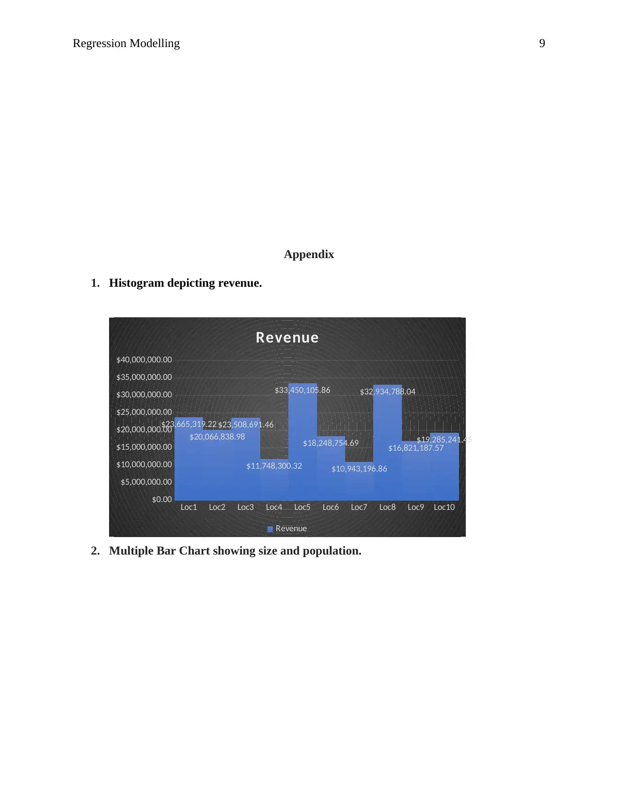
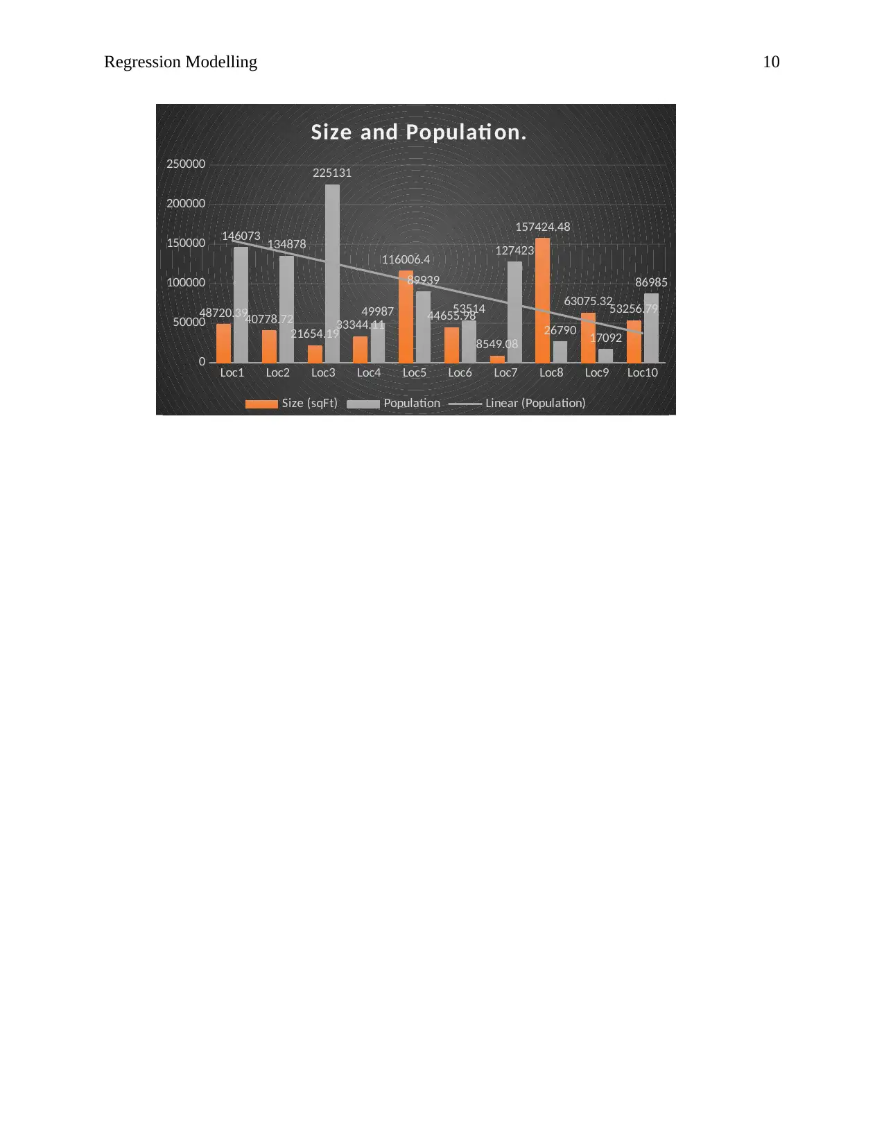
This report presents a multiple linear regression (MLR) analysis to determine factors influencing revenue in Big Grocery stores. The analysis uses data on revenue, store size, and customer population across ten locations. The MLR model, formulated as Revenue = I0 + I1(Size) + I2(Population)+ µ, aims to identify the significant predictors of revenue. The results reveal that both store size and population positively influence revenue, with size having a stronger impact. Statistical outputs, including regression statistics and coefficient tables, are interpreted to assess the model's goodness of fit and the significance of each independent variable. The report also discusses underlying assumptions of the regression model, including linearity, random sampling, and the impact of sample size, and proposes a managerial decision based on the analysis. The conclusion suggests that Big Groceries should prioritize managers who can effectively manage larger store sizes and higher customer populations to maximize revenue.
1 out of 10
Related Documents


Your All-in-One AI-Powered Toolkit for Academic Success.
+13062052269
info@desklib.com
Available 24*7 on WhatsApp / Email
![[object Object]](/_next/static/media/star-bottom.7253800d.svg)
Copyright © 2020–2026 A2Z Services. All Rights Reserved. Developed and managed by ZUCOL.