Regression Analysis and ANOVA Univariate Test for Carbon Emissions Reduction Initiatives

This research project analyzes the impact of the highest level of direct responsibility to climate change and incentives for management of climate change issues on carbon emissions reduction initiatives using regression analysis and ANOVA univariate test.

RESEARCH PROJECT
Data Analysis – Inferential
A. Regression Analysis
Regression Analysis is statistical analysis tool that provides a definition of the way in
which variables in the same set (dataset) relate to one another (Galit, et al., 2018; Howitt
& Cramer, 2010). The variables from the set are divided into independent and dependent
subsets, and the influence of the independent subset on the dependent subset is evaluated
(Claeskens & Hjort, 2008; Szekely & Rizzo, 2009).
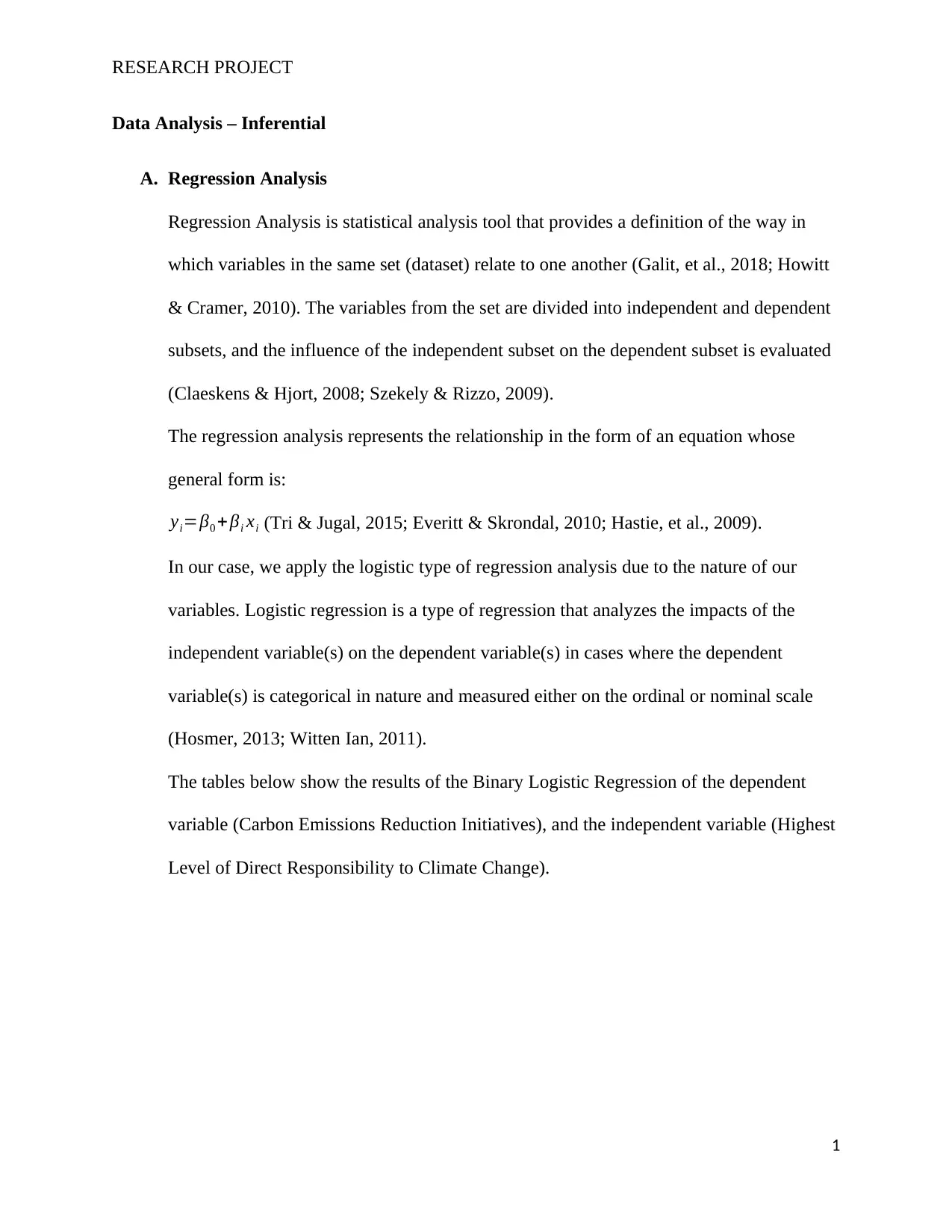
The regression analysis represents the relationship in the form of an equation whose
general form is:
yi=β0 + βi xi (Tri & Jugal, 2015; Everitt & Skrondal, 2010; Hastie, et al., 2009).
In our case, we apply the logistic type of regression analysis due to the nature of our
variables. Logistic regression is a type of regression that analyzes the impacts of the
independent variable(s) on the dependent variable(s) in cases where the dependent
variable(s) is categorical in nature and measured either on the ordinal or nominal scale
(Hosmer, 2013; Witten Ian, 2011).
The tables below show the results of the Binary Logistic Regression of the dependent
variable (Carbon Emissions Reduction Initiatives), and the independent variable (Highest
Level of Direct Responsibility to Climate Change).
1

RESEARCH PROJECT
Table 1: Logistic Regression (Intercept Only Model)
Variables in the Equation
B S.E. Wald df Sig. Exp(B)
Step
0
Constant -2.854 .310 84.742 1 .000 .058
Table 2: Logistic Regression (Overall Model Statistics)
Variables not in the Equation
Score df Sig.
Step
0
Variables CC11Whereisthehighestl
evelofdirectresponsibility
forclimatechang
2.304 1 .129
Overall Statistics 2.304 1 .129
Table 3: Logistic Regression (Model Summary)
Model Summary
Step -2 Log
likelihood
Cox & Snell R
Square
Nagelkerke R
Square
1 82.542a .014 .041
a. Estimation terminated at iteration number 7 because
parameter estimates changed by less than .001.
Table 4: Logistic Regression (Model Statistics)
Variables in the Equation
B S.E. Wald df Sig. Exp(B)
Step
1a
CC11Whereisthehighestle
velofdirectresponsibilityfor
climatechang
1.623 1.072 2.295 1 .130 5.070
Constant -5.962 2.153 7.666 1 .006 .003
a. Variable(s) entered on step 1: CC11Whereisthehighestlevelofdirectresponsibilityforclimatechang.
2

RESEARCH PROJECT
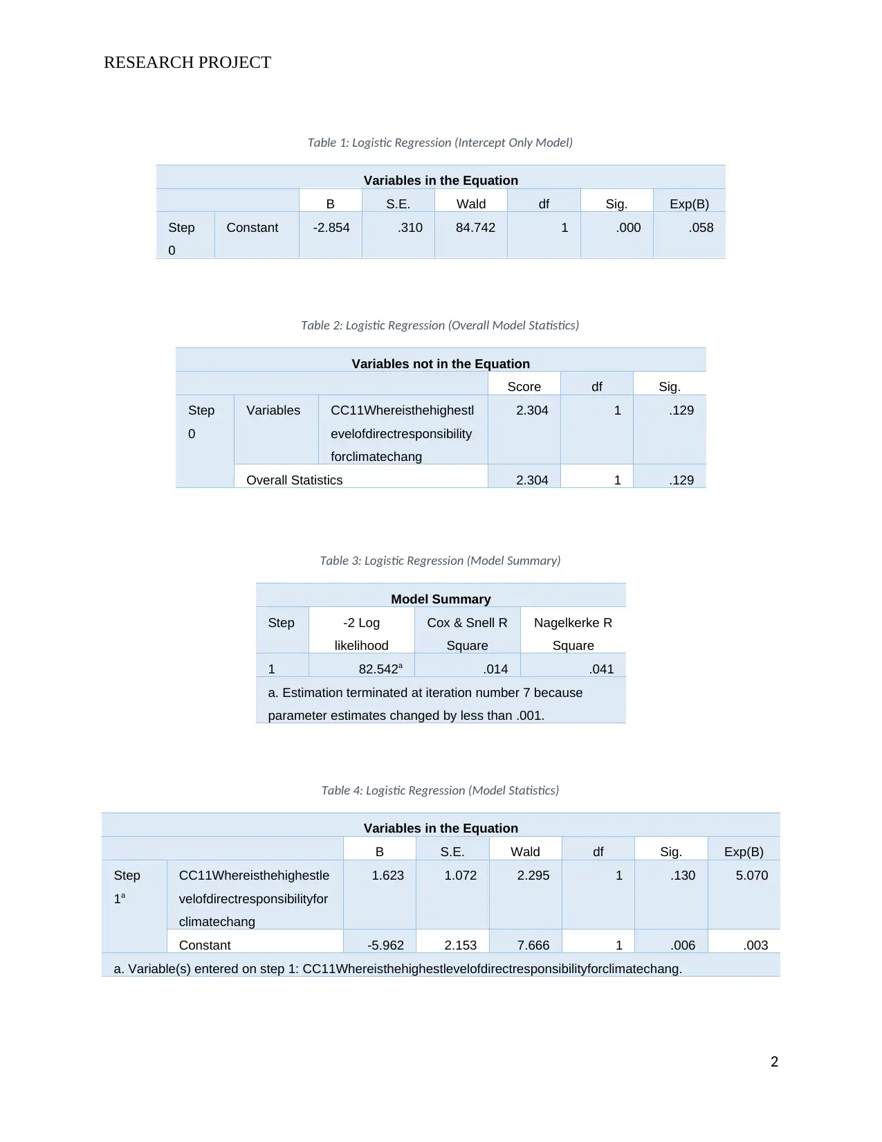
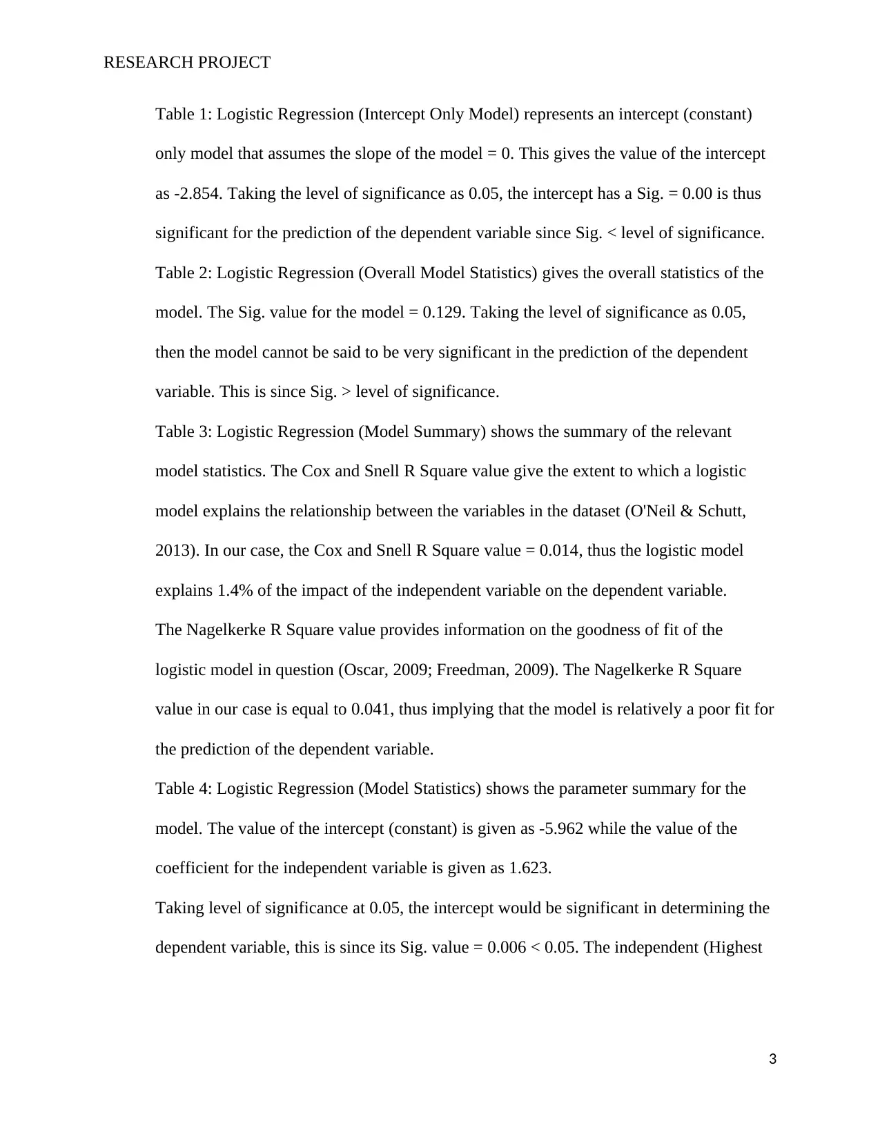
Table 1: Logistic Regression (Intercept Only Model) represents an intercept (constant)
only model that assumes the slope of the model = 0. This gives the value of the intercept
as -2.854. Taking the level of significance as 0.05, the intercept has a Sig. = 0.00 is thus
significant for the prediction of the dependent variable since Sig. < level of significance.
Table 2: Logistic Regression (Overall Model Statistics) gives the overall statistics of the
model. The Sig. value for the model = 0.129. Taking the level of significance as 0.05,
then the model cannot be said to be very significant in the prediction of the dependent
variable. This is since Sig. > level of significance.
Table 3: Logistic Regression (Model Summary) shows the summary of the relevant
model statistics. The Cox and Snell R Square value give the extent to which a logistic
model explains the relationship between the variables in the dataset (O'Neil & Schutt,
2013). In our case, the Cox and Snell R Square value = 0.014, thus the logistic model
explains 1.4% of the impact of the independent variable on the dependent variable.
The Nagelkerke R Square value provides information on the goodness of fit of the
logistic model in question (Oscar, 2009; Freedman, 2009). The Nagelkerke R Square
value in our case is equal to 0.041, thus implying that the model is relatively a poor fit for
the prediction of the dependent variable.
Table 4: Logistic Regression (Model Statistics) shows the parameter summary for the
model. The value of the intercept (constant) is given as -5.962 while the value of the
coefficient for the independent variable is given as 1.623.
Taking level of significance at 0.05, the intercept would be significant in determining the
dependent variable, this is since its Sig. value = 0.006 < 0.05. The independent (Highest
3

RESEARCH PROJECT
Level of Responsibility to Climate Change) however, is not significant in determining the
dependent variable, since its Sig. value = 0.13 > 0.05.
The tables below show the results of the Binary Logistic Regression of the dependent
variable (Carbon Emissions Reduction Initiatives), the independent variable (Highest
Level of Direct Responsibility to Climate Change) and the moderating variable (Incentive
for Management of Climate Change Issues).
Table 5: Logistic Regression with Moderating Variable (Intercept Only Model)
Variables in the Equation
B S.E. Wald df Sig. Exp(B)
Step
0
Constant -2.854 .310 84.742 1 .000 .058
Table 6: Logistic Regression with Moderating Variable (Overall Model Statistics)
Variables not in the Equation
Score df Sig.
Step
0
Variables CC11Whereisthehighestl
evelofdirectresponsibility
forclimatechang
2.304 1 .129
CC12Doyouprovideincen
tivesforthemanagemento
fclimatechangeissues
10.119 1 .001
Overall Statistics 13.059 2 .001
Table 7: Logistic Regression with Moderating Variable (Model Summary)
Model Summary
Step -2 Log
likelihood
Cox & Snell R
Square
Nagelkerke R
Square
1 69.691a .075 .217
4

RESEARCH PROJECT
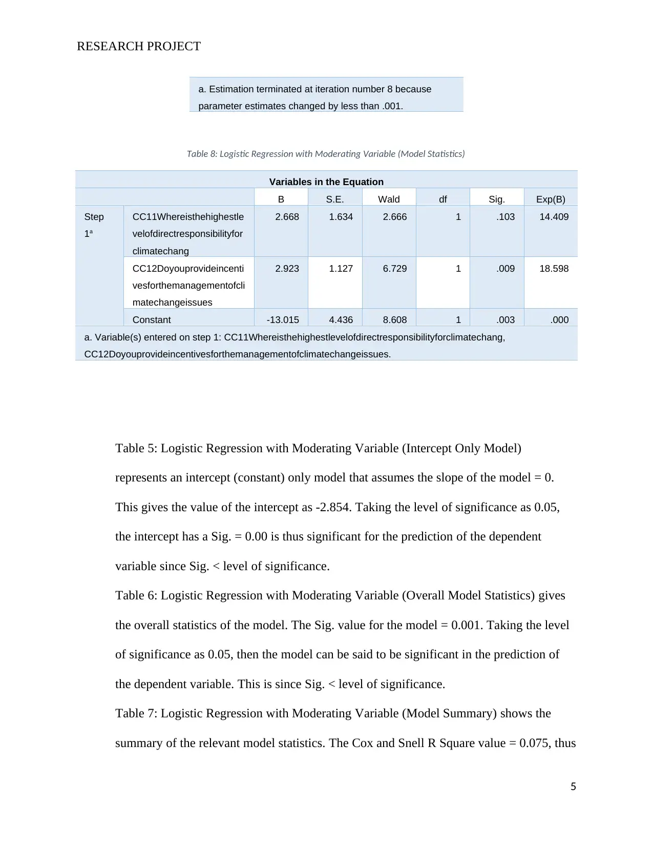
a. Estimation terminated at iteration number 8 because
parameter estimates changed by less than .001.
Table 8: Logistic Regression with Moderating Variable (Model Statistics)
Variables in the Equation
B S.E. Wald df Sig. Exp(B)
Step
1a
CC11Whereisthehighestle
velofdirectresponsibilityfor
climatechang
2.668 1.634 2.666 1 .103 14.409
CC12Doyouprovideincenti
vesforthemanagementofcli
matechangeissues
2.923 1.127 6.729 1 .009 18.598
Constant -13.015 4.436 8.608 1 .003 .000
a. Variable(s) entered on step 1: CC11Whereisthehighestlevelofdirectresponsibilityforclimatechang,
CC12Doyouprovideincentivesforthemanagementofclimatechangeissues.
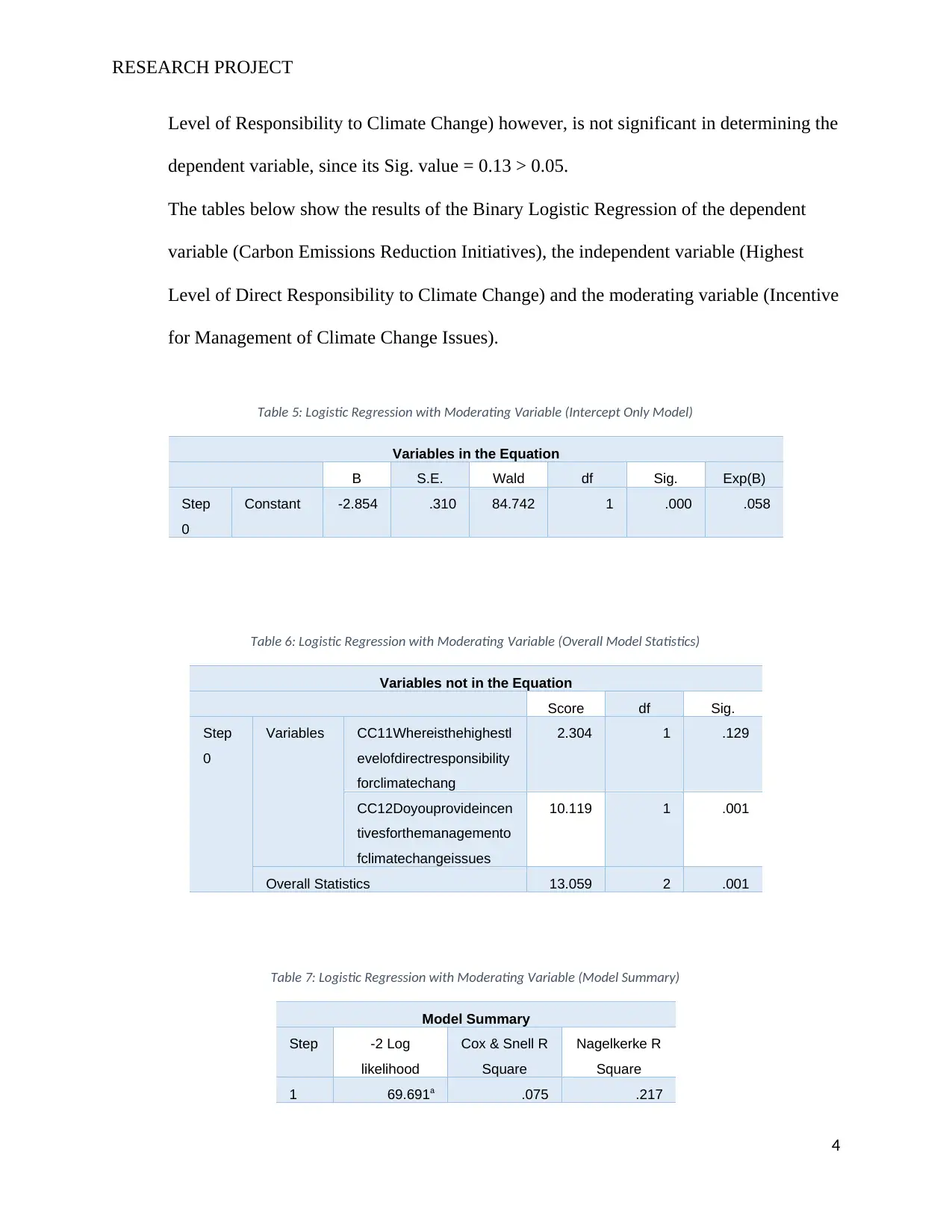
Table 5: Logistic Regression with Moderating Variable (Intercept Only Model)
represents an intercept (constant) only model that assumes the slope of the model = 0.
This gives the value of the intercept as -2.854. Taking the level of significance as 0.05,
the intercept has a Sig. = 0.00 is thus significant for the prediction of the dependent
variable since Sig. < level of significance.
Table 6: Logistic Regression with Moderating Variable (Overall Model Statistics) gives
the overall statistics of the model. The Sig. value for the model = 0.001. Taking the level
of significance as 0.05, then the model can be said to be significant in the prediction of
the dependent variable. This is since Sig. < level of significance.
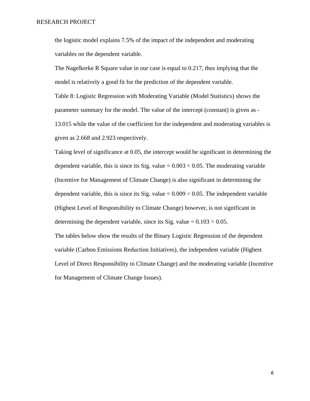
Table 7: Logistic Regression with Moderating Variable (Model Summary) shows the
summary of the relevant model statistics. The Cox and Snell R Square value = 0.075, thus
5

RESEARCH PROJECT
the logistic model explains 7.5% of the impact of the independent and moderating
variables on the dependent variable.
The Nagelkerke R Square value in our case is equal to 0.217, thus implying that the
model is relatively a good fit for the prediction of the dependent variable.
Table 8: Logistic Regression with Moderating Variable (Model Statistics) shows the
parameter summary for the model. The value of the intercept (constant) is given as -
13.015 while the value of the coefficient for the independent and moderating variables is
given as 2.668 and 2.923 respectively.
Taking level of significance at 0.05, the intercept would be significant in determining the
dependent variable, this is since its Sig. value = 0.003 < 0.05. The moderating variable
(Incentive for Management of Climate Change) is also significant in determining the
dependent variable, this is since its Sig. value = 0.009 < 0.05. The independent variable
(Highest Level of Responsibility to Climate Change) however, is not significant in
determining the dependent variable, since its Sig. value = 0.103 > 0.05.
The tables below show the results of the Binary Logistic Regression of the dependent
variable (Carbon Emissions Reduction Initiatives), the independent variable (Highest
Level of Direct Responsibility to Climate Change) and the moderating variable (Incentive
for Management of Climate Change Issues).
6

RESEARCH PROJECT
B. ANOVA Univariate Test
The Analysis of Variance (commonly ANOVA) test is a statistical test that is applied in
order to determine the significance of the results of the study carried out on research
variables (Babbie, 2010; Barbara & Susan, 2014).
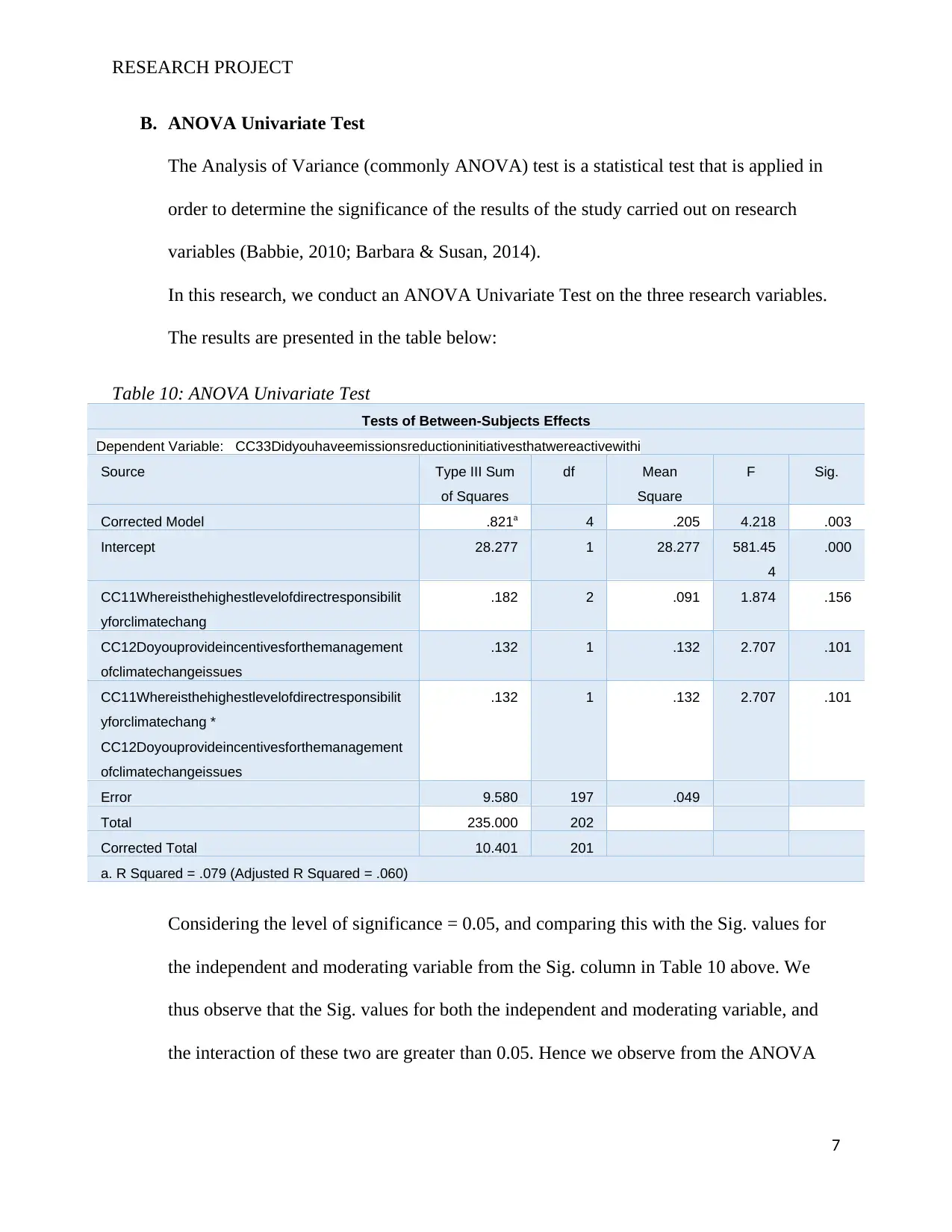
In this research, we conduct an ANOVA Univariate Test on the three research variables.
The results are presented in the table below:
Table 10: ANOVA Univariate Test
Tests of Between-Subjects Effects
Dependent Variable: CC33Didyouhaveemissionsreductioninitiativesthatwereactivewithi
Source Type III Sum
of Squares
df Mean
Square
F Sig.
Corrected Model .821a 4 .205 4.218 .003
Intercept 28.277 1 28.277 581.45
4
.000
CC11Whereisthehighestlevelofdirectresponsibilit
yforclimatechang
.182 2 .091 1.874 .156
CC12Doyouprovideincentivesforthemanagement
ofclimatechangeissues
.132 1 .132 2.707 .101
CC11Whereisthehighestlevelofdirectresponsibilit
yforclimatechang *
CC12Doyouprovideincentivesforthemanagement
ofclimatechangeissues
.132 1 .132 2.707 .101
Error 9.580 197 .049
Total 235.000 202
Corrected Total 10.401 201
a. R Squared = .079 (Adjusted R Squared = .060)
Considering the level of significance = 0.05, and comparing this with the Sig. values for
the independent and moderating variable from the Sig. column in Table 10 above. We
thus observe that the Sig. values for both the independent and moderating variable, and
the interaction of these two are greater than 0.05. Hence we observe from the ANOVA
7

RESEARCH PROJECT
univariate test that neither the independent nor the moderating variables are significant in
determining the dependent variable.
Hypothesis Testing
The hypothesis in this research is;
H0: The Carbon Emissions Reduction Initiatives of a company are affected by the Highest Level
of Direct Responsibility to Climate Change in the same company.
H1: The Carbon Emissions Reduction Initiatives of a company is not affected by the Highest
Level of Direct Responsibility to Climate Change in the same company.
Decision Rule: We consider the regression analysis results presented in Table 4: Logistic
Regression (Model Statistics). From this table we observe that the Sig. value of the independent
(Highest Level of Responsibility to Climate Change) = 0.13. Taking the level of significance as
0.05, the independent (Highest Level of Responsibility to Climate Change) does not significantly
affect the dependent variable, since its Sig. value = 0.13 > 0.05.
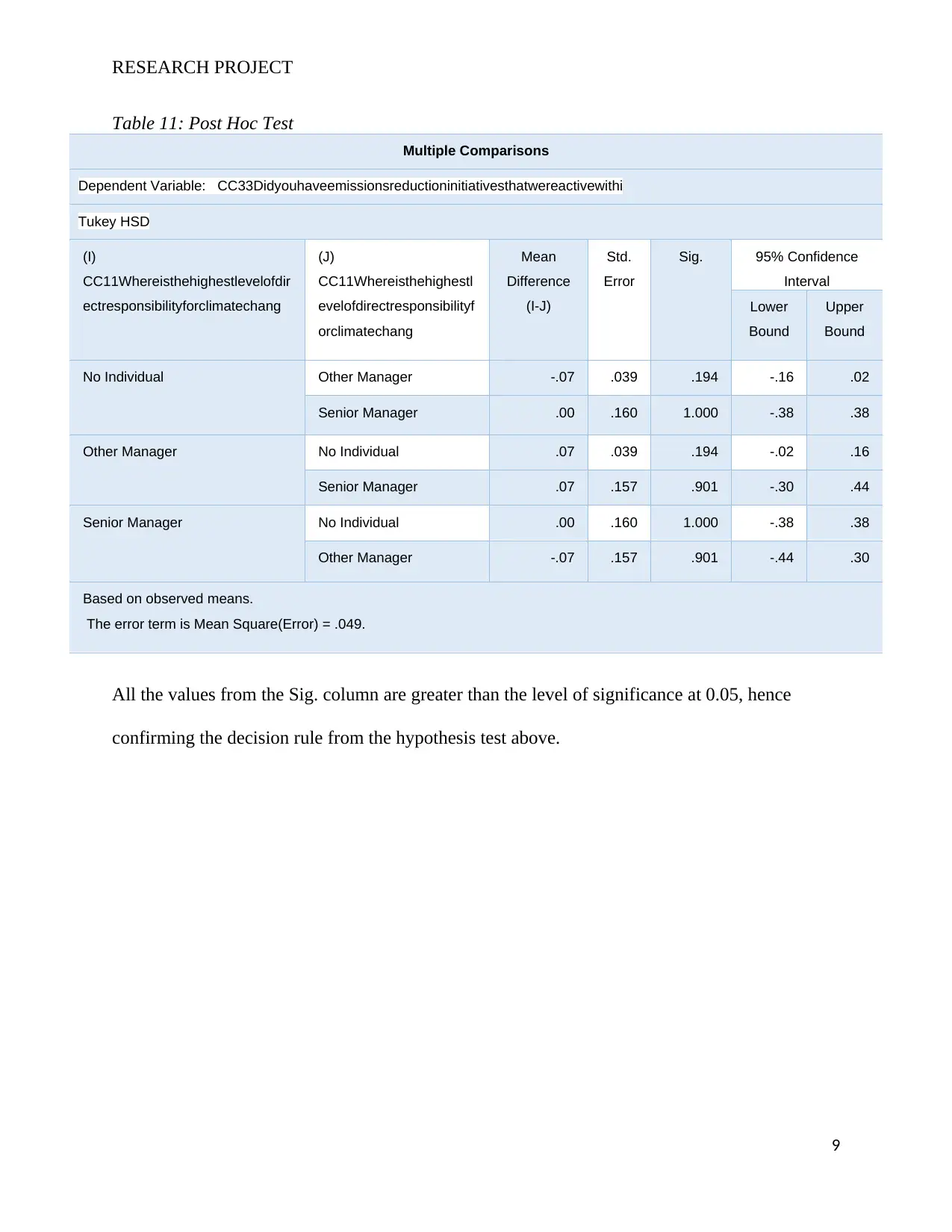
We also observe the same from the Post Hoc Test for the variables, we obtain the results in the
table below from the test:
8

RESEARCH PROJECT
Table 11: Post Hoc Test
Multiple Comparisons
Dependent Variable: CC33Didyouhaveemissionsreductioninitiativesthatwereactivewithi
Tukey HSD
(I)
CC11Whereisthehighestlevelofdir
ectresponsibilityforclimatechang
(J)
CC11Whereisthehighestl
evelofdirectresponsibilityf
orclimatechang
Mean
Difference
(I-J)
Std.
Error
Sig. 95% Confidence
Interval
Lower
Bound
Upper
Bound
No Individual Other Manager -.07 .039 .194 -.16 .02
Senior Manager .00 .160 1.000 -.38 .38
Other Manager No Individual .07 .039 .194 -.02 .16
Senior Manager .07 .157 .901 -.30 .44
Senior Manager No Individual .00 .160 1.000 -.38 .38
Other Manager -.07 .157 .901 -.44 .30
Based on observed means.
The error term is Mean Square(Error) = .049.
All the values from the Sig. column are greater than the level of significance at 0.05, hence
confirming the decision rule from the hypothesis test above.
9

RESEARCH PROJECT
Discussion
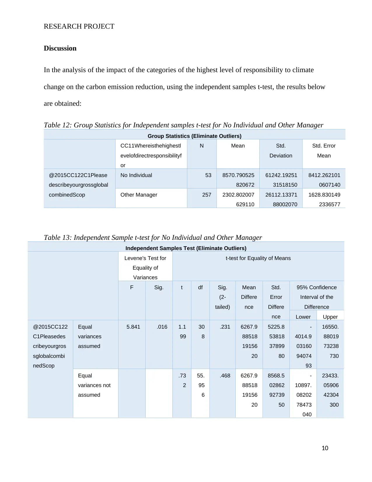
In the analysis of the impact of the categories of the highest level of responsibility to climate
change on the carbon emission reduction, using the independent samples t-test, the results below
are obtained:
Table 12: Group Statistics for Independent samples t-test for No Individual and Other Manager
Group Statistics (Eliminate Outliers)
CC11Whereisthehighestl
evelofdirectresponsibilityf
or
N Mean Std.
Deviation
Std. Error
Mean
@2015CC122C1Please
describeyourgrossglobal
combinedScop
No Individual 53 8570.790525
820672
61242.19251
31518150
8412.262101
0607140
Other Manager 257 2302.802007
629110
26112.13371
88002070
1628.830149
2336577
Table 13: Independent Sample t-test for No Individual and Other Manager
Independent Samples Test (Eliminate Outliers)
Levene's Test for
Equality of
Variances
t-test for Equality of Means
F Sig. t df Sig.
(2-
tailed)
Mean
Differe
nce
Std.
Error
Differe
nce
95% Confidence
Interval of the
Difference
Lower Upper
@2015CC122
C1Pleasedes
cribeyourgros
sglobalcombi
nedScop
Equal
variances
assumed
5.841 .016 1.1
99
30
8
.231 6267.9
88518
19156
20
5225.8
53818
37899
80
-
4014.9
03160
94074
93
16550.
88019
73238
730
Equal
variances not
assumed
.73
2
55.
95
6
.468 6267.9
88518
19156
20
8568.5
02862
92739
50
-
10897.
08202
78473
040
23433.
05906
42304
300
10

RESEARCH PROJECT
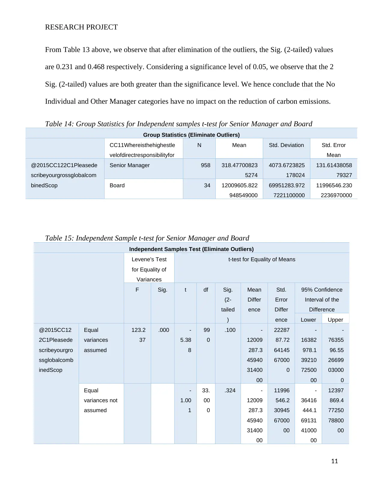
From Table 13 above, we observe that after elimination of the outliers, the Sig. (2-tailed) values
are 0.231 and 0.468 respectively. Considering a significance level of 0.05, we observe that the 2
Sig. (2-tailed) values are both greater than the significance level. We hence conclude that the No
Individual and Other Manager categories have no impact on the reduction of carbon emissions.
Table 14: Group Statistics for Independent samples t-test for Senior Manager and Board
Group Statistics (Eliminate Outliers)
CC11Whereisthehighestle
velofdirectresponsibilityfor
N Mean Std. Deviation Std. Error
Mean
@2015CC122C1Pleasede
scribeyourgrossglobalcom
binedScop
Senior Manager 958 318.47700823
5274
4073.6723825
178024
131.61438058
79327
Board 34 12009605.822
948549000
69951283.972
7221100000
11996546.230
2236970000
Table 15: Independent Sample t-test for Senior Manager and Board
Independent Samples Test (Eliminate Outliers)
Levene's Test
for Equality of
Variances
t-test for Equality of Means
F Sig. t df Sig.
(2-
tailed
)
Mean
Differ
ence
Std.
Error
Differ
ence
95% Confidence
Interval of the
Difference
Lower Upper
@2015CC12
2C1Pleasede
scribeyourgro
ssglobalcomb
inedScop
Equal
variances
assumed
123.2
37
.000 -
5.38
8
99
0
.100 -
12009
287.3
45940
31400
00
22287
87.72
64145
67000
0
-
16382
978.1
39210
72500
00
-
76355
96.55
26699
03000
0
Equal
variances not
assumed
-
1.00
1
33.
00
0
.324 -
12009
287.3
45940
31400
00
11996
546.2
30945
67000
00
-
36416
444.1
69131
41000
00
12397
869.4
77250
78800
00
11

RESEARCH PROJECT
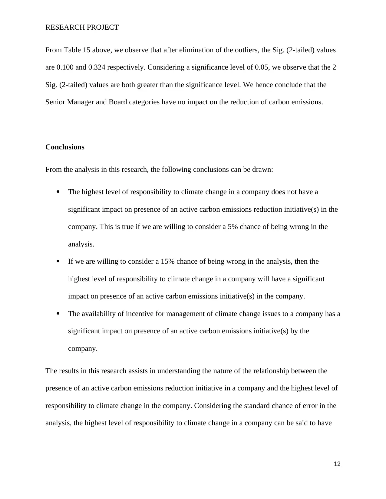
From Table 15 above, we observe that after elimination of the outliers, the Sig. (2-tailed) values
are 0.100 and 0.324 respectively. Considering a significance level of 0.05, we observe that the 2
Sig. (2-tailed) values are both greater than the significance level. We hence conclude that the
Senior Manager and Board categories have no impact on the reduction of carbon emissions.
Conclusions
From the analysis in this research, the following conclusions can be drawn:
 The highest level of responsibility to climate change in a company does not have a
significant impact on presence of an active carbon emissions reduction initiative(s) in the
company. This is true if we are willing to consider a 5% chance of being wrong in the
analysis.
 If we are willing to consider a 15% chance of being wrong in the analysis, then the
highest level of responsibility to climate change in a company will have a significant
impact on presence of an active carbon emissions initiative(s) in the company.
 The availability of incentive for management of climate change issues to a company has a
significant impact on presence of an active carbon emissions initiative(s) by the
company.
The results in this research assists in understanding the nature of the relationship between the
presence of an active carbon emissions reduction initiative in a company and the highest level of
responsibility to climate change in the company. Considering the standard chance of error in the
analysis, the highest level of responsibility to climate change in a company can be said to have
12

RESEARCH PROJECT
no significant effect on the presence of an active carbon emissions reduction initiative in the
company.
This would in turn imply, in the practical sense, that a company having the carbon emissions
reduction task assigned to a high level office, individual or board does not mean that the
company will automatically pursue carbon emissions reduction initiatives.
Based on the results of the analysis in this research, I would recommend that more attention be
given to the actual presence and implementation of the carbon emissions reduction initiatives
rather than who is in charge of developing and implementing the initiatives. Then, the initiatives
can be observed as to whether they are resulting to actual reductions in the carbon emissions.
Limitations
 The inferences drawn from this research would be more reliable if there was a bigger
sample size. The sample size of 220 observations resulted from exclusion of entries that
had anomalies. If the anomalies were absent, it would have improved the reliability of the
study.
 The data contained numerous null entries, and can therefore be said to have been
incomplete. This limited the sample size that could be considered for the study.
 Since the study largely made use of a small sample size, generalizing the results from the
research for entire industrial sectors and all countries globally would be inaccurate.
13

RESEARCH PROJECT
Further Research
In order to improve on the findings made in this research, further analysis has to be done. This
should be done on a dataset that can be considered as complete without missing entries. The
completeness of the dataset would afford the research a sufficient sample size for proper
analysis. Consideration should also be given to inclusion of more independent variables to
broaden the research.
Also comparison of findings on the variable interaction should be done for the datasets of
different years (for 2011, base year, and say 2015), for the variables in this research and
additional ones such as the carbon emission reduction. The table below shows an overview of
such a comparison giving consideration to 2011, the base year, and the year 2015 using a paired
sample t-test.
Table 16: Paired sample t-test for Carbon emission reduction for years 2011 and 2015
Paired Samples Test
Paired Differences t df Sig. (2-
tailed)Mean Std.
Deviation
Std.
Error
Mean
95% Confidence
Interval of the
Difference
Lower Upper
Pair 1 @2011CC122
C1Pleasedescr
ibeyourgrossgl
obalcombinedS
cop -
@2015CC122
C1Pleasedescr
ibeyourgrossgl
obalcombinedS
cop
2483222.
5036123
088000
6901770
2.608551
3500000
1909804.
4914415
180000
-
1263400.
3889318
835000
6229845.
3961565
010000
1.30
0
1305 .194
14

RESEARCH PROJECT
References
Babbie, E. R., 2010. The Practice of Social Research 12th edition. 1st ed. Belmont, CA:
Wadsworth Cengage.
Barbara, I. & Susan, D., 2014. Introductory Statistics. 1st ed. New York: OpenStax CNX.
Claeskens, G. & Hjort, N. L., 2008. Model Selection and Model Averaging. 1st ed. London:
Cambridge University Press.
Everitt, B. S. & Skrondal, A., 2010. Cambridge Dictionary of Statistics. 4th ed. London:
Cambridge University Press.
Freedman, D. A., 2009. Statistical Models: Theory and Practice. 1st ed. London: Cambridge
University Press.
Galit, S. et al., 2018. Data Mining for Business Analytics. 1st ed. New Delhi: John Wiley &
Sons, Inc..
Hastie, T., Tibshir, R. & Jerome, H., 2009. The Elements of Statistical Learning. 2nd ed. New
York: Springer.
Hosmer, D., 2013. Applied Logistic Regression. 1 ed. Hoboken, New Jersey: Wiley.
Howitt, D. & Cramer, D., 2010. Introduction to Descriptive Statistics in Psycology, 5th Edition.
New York: Prentice Hall.
O'Neil, C. & Schutt, R., 2013. Doing Data Science. 3rd ed. London: O'Reily.
Oscar, M., 2009. A data mining and knowledge discovery process model. 1st ed. Vienna: Julio
Ponce.
15

RESEARCH PROJECT
Szekely, G. J. & Rizzo, M. L., 2009. Brownian Distance Covariance. Annals of Applied
Statistics, 3(4), pp. 1233-1303.
Tri, D. & Jugal, K., 2015. Select Machine Learning Algorithms Using Regression Models, s.l.:
2015 IEEE Conference.
Witten Ian, 2011. Data Mining: Practical Machine Learning Tools. s.l.:Elsevier.
16