ECOM90009 Quantitative Methods: Regression, Forecasting & Housing Data
VerifiedAdded on 2023/06/03
|14
|1990
|464
Homework Assignment
AI Summary
This assignment solution for ECOM90009 Quantitative Methods for Business focuses on regression analysis and time series forecasting. It includes a preliminary analysis of a regression model with descriptive statistics, correlation coefficients, and scatter diagrams to assess the relationships between variables. The solution also presents a regression model for predicting margin, discusses the significance of error terms, and evaluates the model's overall significance. Furthermore, it explores a parsimonious regression model and compares its performance against the original model. The assignment also covers time series analysis, including average forecasts, multiplicative time series models, and linear and quadratic forecasts for housing starts in Victoria, ultimately recommending the seasonal indices model for future predictions.

Subject Code: Subject Name:
Assignment Number: Workshop Day and Time:
Tutor Name:
Student ID Number Student Name
1.
2.
3.
4.
Assignment Number: Workshop Day and Time:
Tutor Name:
Student ID Number Student Name
1.
2.
3.
4.
Paraphrase This Document
Need a fresh take? Get an instant paraphrase of this document with our AI Paraphraser
Question 1
a. Preliminary analysis of the regression model
1) Descriptive statistics
Descriptive statistics
Margin Number Nearest Office Space Enrolment Income Distance Quality
Mean 46.4175 Mean 2977.616667 Mean 2.305833333 Mean 50.59333333 Mean 16.21416667 Mean 39.2 Mean 11.2495 Mean 0.566666667
Standard Error 0.712709414 Standard Error 41.70926984 Standard Error 0.078512928 Standard Error 1.542685703 Standard Error 0.39983767 Standard Error 0.432664858 Standard Error 0.445172422 Standard Error 0.045425676
Median 46.9 Median 2971 Median 2.3 Median 49.65 Median 16 Median 39 Median 12.08 Median 1
Mode 54.4 Mode 3003 Mode 2.2 Mode 44.9 Mode 15.5 Mode 40 Mode 12.16 Mode 1
Standard Deviation 7.807340464 Standard Deviation 456.902159 Standard Deviation 0.860066036 Standard Deviation 16.89927517 Standard Deviation 4.380002222 Standard Deviation 4.739606054 Standard Deviation 4.87661955 Standard Deviation 0.497613352
Sample Variance 60.95456513 Sample Variance 208759.5829 Sample Variance 0.739713585 Sample Variance 285.5855014 Sample Variance 19.18441947 Sample Variance 22.46386555 Sample Variance 23.78141824 Sample Variance 0.247619048
Kurtosis -0.392893447 Kurtosis 0.236234585 Kurtosis -0.470697081 Kurtosis -0.318372074 Kurtosis -0.503259346 Kurtosis -0.510651311 Kurtosis -0.46710657 Kurtosis -1.958680173
Skewness -0.162069201 Skewness -0.261272802 Skewness 0.015427532 Skewness -0.012656933 Skewness 0.038526881 Skewness 0.008437444 Skewness -0.036439358 Skewness -0.272487103
Range 39.2 Range 2601 Range 4.1 Range 73.5 Range 20.5 Range 22 Range 22.72 Range 1
Minimum 27.3 Minimum 1613 Minimum 0.1 Minimum 14 Minimum 6 Minimum 28 Minimum 0.32 Minimum 0
Maximum 66.5 Maximum 4214 Maximum 4.2 Maximum 87.5 Maximum 26.5 Maximum 50 Maximum 23.04 Maximum 1
Sum 5570.1 Sum 357314 Sum 276.7 Sum 6071.2 Sum 1945.7 Sum 4704 Sum 1349.94 Sum 68
Count 120 Count 120 Count 120 Count 120 Count 120 Count 120 Count 120 Count 120
Largest(1) 66.5 Largest(1) 4214 Largest(1) 4.2 Largest(1) 87.5 Largest(1) 26.5 Largest(1) 50 Largest(1) 23.04 Largest(1) 1
Smallest(1) 27.3 Smallest(1) 1613 Smallest(1) 0.1 Smallest(1) 14 Smallest(1) 6 Smallest(1) 28 Smallest(1) 0.32 Smallest(1) 0
Confidence Level(95.0%) 1.411235823 Confidence Level(95.0%) 82.58852007 Confidence Level(95.0%) 0.155463439 Confidence Level(95.0%) 3.05467177 Confidence Level(95.0%) 0.791718521 Confidence Level(95.0%) 0.856719632 Confidence Level(95.0%) 0.881485858 Confidence Level(95.0%) 0.089947376
From the descriptive statistics the appropriate estimate of the Margin will be
obtained from the mean, this gives a value of 46.4175. This value can be affected
with presence of outliers hence leading to inaccurate estimation of the margin
value.
The skewness of the Income data is 0.0084, this indicates that the data is
symmetrically distributed.
The sum of the quality variable indicates the number of motels that have been
built or extensively renovated in the past 6 years.
2) Set of correlation coefficient
Correlation coeffi cient
Margin Number Nearest Office Space Enrolment Income Distance Quality
Margin 1
Number -0.487627077 1
Nearest 0.188492588 0.064537585 1
Offi ce Space 0.588401934 -0.11525533 0.189820646 1
Enrolment 0.128399133 -0.059278379 0.038279504 0.035072974 1
Income 0.208150784 0.071863738 -0.051413296 0.117281667 -0.107853908 1
Distance -0.13058048 0.120497632 0.179926405 0.019342162 0.08452925 -0.103475854 1
Quality 0.399745297 -0.15268135 0.096276576 0.269762533 0.093060199 0.022803355 -0.149064745 1
Testing the hypothesis
H0 ; ρ=0
Vs
H0 ; ρ≠ 0
z=r∗√n
α=0.05
Using the indicated formula, we can derive a table of z statistics as shown below
a. Preliminary analysis of the regression model
1) Descriptive statistics
Descriptive statistics
Margin Number Nearest Office Space Enrolment Income Distance Quality
Mean 46.4175 Mean 2977.616667 Mean 2.305833333 Mean 50.59333333 Mean 16.21416667 Mean 39.2 Mean 11.2495 Mean 0.566666667
Standard Error 0.712709414 Standard Error 41.70926984 Standard Error 0.078512928 Standard Error 1.542685703 Standard Error 0.39983767 Standard Error 0.432664858 Standard Error 0.445172422 Standard Error 0.045425676
Median 46.9 Median 2971 Median 2.3 Median 49.65 Median 16 Median 39 Median 12.08 Median 1
Mode 54.4 Mode 3003 Mode 2.2 Mode 44.9 Mode 15.5 Mode 40 Mode 12.16 Mode 1
Standard Deviation 7.807340464 Standard Deviation 456.902159 Standard Deviation 0.860066036 Standard Deviation 16.89927517 Standard Deviation 4.380002222 Standard Deviation 4.739606054 Standard Deviation 4.87661955 Standard Deviation 0.497613352
Sample Variance 60.95456513 Sample Variance 208759.5829 Sample Variance 0.739713585 Sample Variance 285.5855014 Sample Variance 19.18441947 Sample Variance 22.46386555 Sample Variance 23.78141824 Sample Variance 0.247619048
Kurtosis -0.392893447 Kurtosis 0.236234585 Kurtosis -0.470697081 Kurtosis -0.318372074 Kurtosis -0.503259346 Kurtosis -0.510651311 Kurtosis -0.46710657 Kurtosis -1.958680173
Skewness -0.162069201 Skewness -0.261272802 Skewness 0.015427532 Skewness -0.012656933 Skewness 0.038526881 Skewness 0.008437444 Skewness -0.036439358 Skewness -0.272487103
Range 39.2 Range 2601 Range 4.1 Range 73.5 Range 20.5 Range 22 Range 22.72 Range 1
Minimum 27.3 Minimum 1613 Minimum 0.1 Minimum 14 Minimum 6 Minimum 28 Minimum 0.32 Minimum 0
Maximum 66.5 Maximum 4214 Maximum 4.2 Maximum 87.5 Maximum 26.5 Maximum 50 Maximum 23.04 Maximum 1
Sum 5570.1 Sum 357314 Sum 276.7 Sum 6071.2 Sum 1945.7 Sum 4704 Sum 1349.94 Sum 68
Count 120 Count 120 Count 120 Count 120 Count 120 Count 120 Count 120 Count 120
Largest(1) 66.5 Largest(1) 4214 Largest(1) 4.2 Largest(1) 87.5 Largest(1) 26.5 Largest(1) 50 Largest(1) 23.04 Largest(1) 1
Smallest(1) 27.3 Smallest(1) 1613 Smallest(1) 0.1 Smallest(1) 14 Smallest(1) 6 Smallest(1) 28 Smallest(1) 0.32 Smallest(1) 0
Confidence Level(95.0%) 1.411235823 Confidence Level(95.0%) 82.58852007 Confidence Level(95.0%) 0.155463439 Confidence Level(95.0%) 3.05467177 Confidence Level(95.0%) 0.791718521 Confidence Level(95.0%) 0.856719632 Confidence Level(95.0%) 0.881485858 Confidence Level(95.0%) 0.089947376
From the descriptive statistics the appropriate estimate of the Margin will be
obtained from the mean, this gives a value of 46.4175. This value can be affected
with presence of outliers hence leading to inaccurate estimation of the margin
value.
The skewness of the Income data is 0.0084, this indicates that the data is
symmetrically distributed.
The sum of the quality variable indicates the number of motels that have been
built or extensively renovated in the past 6 years.
2) Set of correlation coefficient
Correlation coeffi cient
Margin Number Nearest Office Space Enrolment Income Distance Quality
Margin 1
Number -0.487627077 1
Nearest 0.188492588 0.064537585 1
Offi ce Space 0.588401934 -0.11525533 0.189820646 1
Enrolment 0.128399133 -0.059278379 0.038279504 0.035072974 1
Income 0.208150784 0.071863738 -0.051413296 0.117281667 -0.107853908 1
Distance -0.13058048 0.120497632 0.179926405 0.019342162 0.08452925 -0.103475854 1
Quality 0.399745297 -0.15268135 0.096276576 0.269762533 0.093060199 0.022803355 -0.149064745 1
Testing the hypothesis
H0 ; ρ=0
Vs
H0 ; ρ≠ 0
z=r∗√n
α=0.05
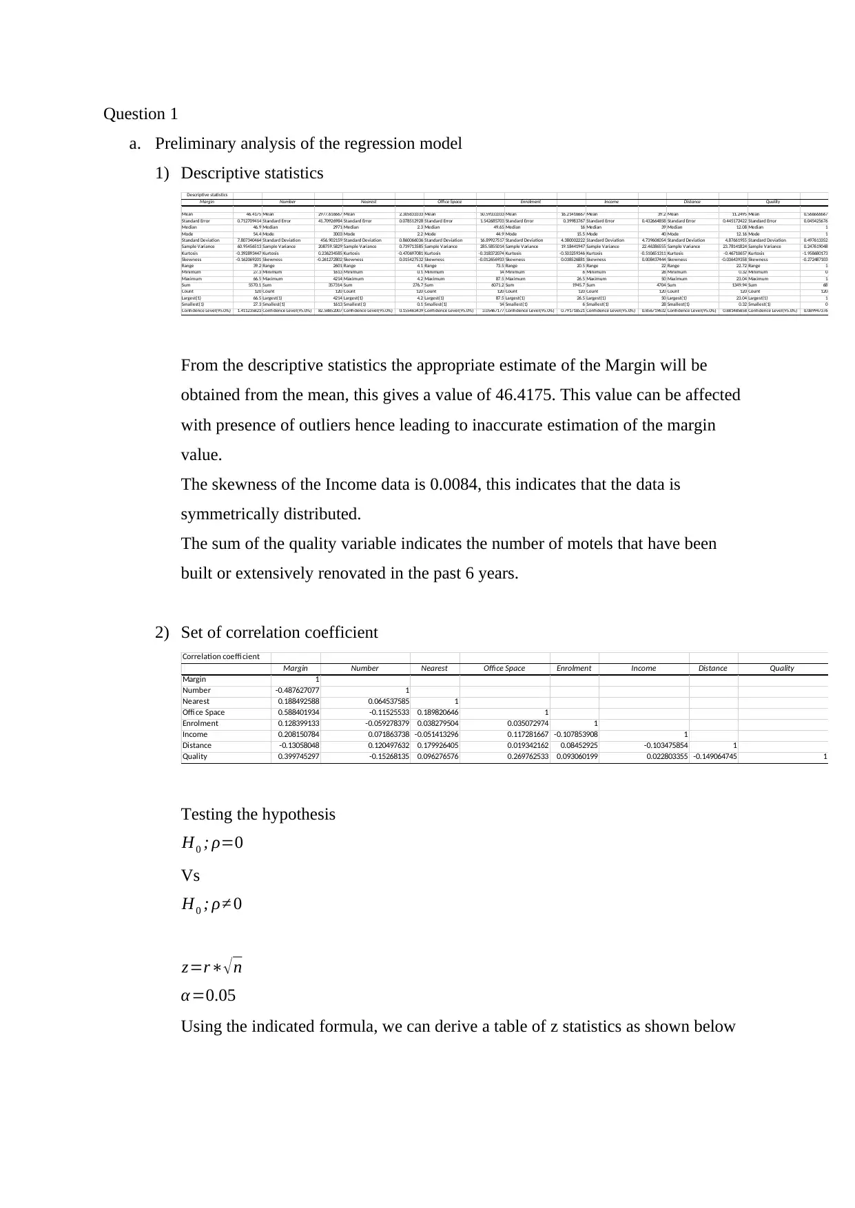
Using the indicated formula, we can derive a table of z statistics as shown below
Obtaining the Z statistics
Margin Number Nearest Office Space Enrolment Income Distance Quality
Margin 10.95445115
Number -5.341686996 10.95445115
Nearest 2.064832851 0.706973821 10.95445115
Offi ce Space 6.445620243 -1.262558883 2.079380997 10.95445115
Enrolment 1.406542032 -0.649362112 0.419330958 0.384205176 10.95445115
Income 2.280177596 0.78722781 -0.563204437 1.284756296 -1.18148037 10.95445115
Distance -1.430437485 1.319985424 1.970995018 0.211882774 0.925971539 -1.133521192 10.95445115
Quality 4.378990325 -1.672540386 1.054657044 2.95510049 1.019423402 0.249798235 -1.632922462 10.95445115
At 5% significance level
We reject the null hypothesis if the value of the z statistics is less than 0.05 and
fail to reject otherwise.
From the tables calculated above the following pairs of variables can be
concluded to have a significant linear relationship.
Margin and (Nearest, Office space, Enrolment, Income, Quality)
Number and (Nearest, Income, Distance)
Nearest and (Office space, Enrolment, distance, Quality)
Office space and (Enrolment, Income, Distance, Quality)
Enrolment and (Distance, Quality)
Income and quality
3) Scatter diagrams
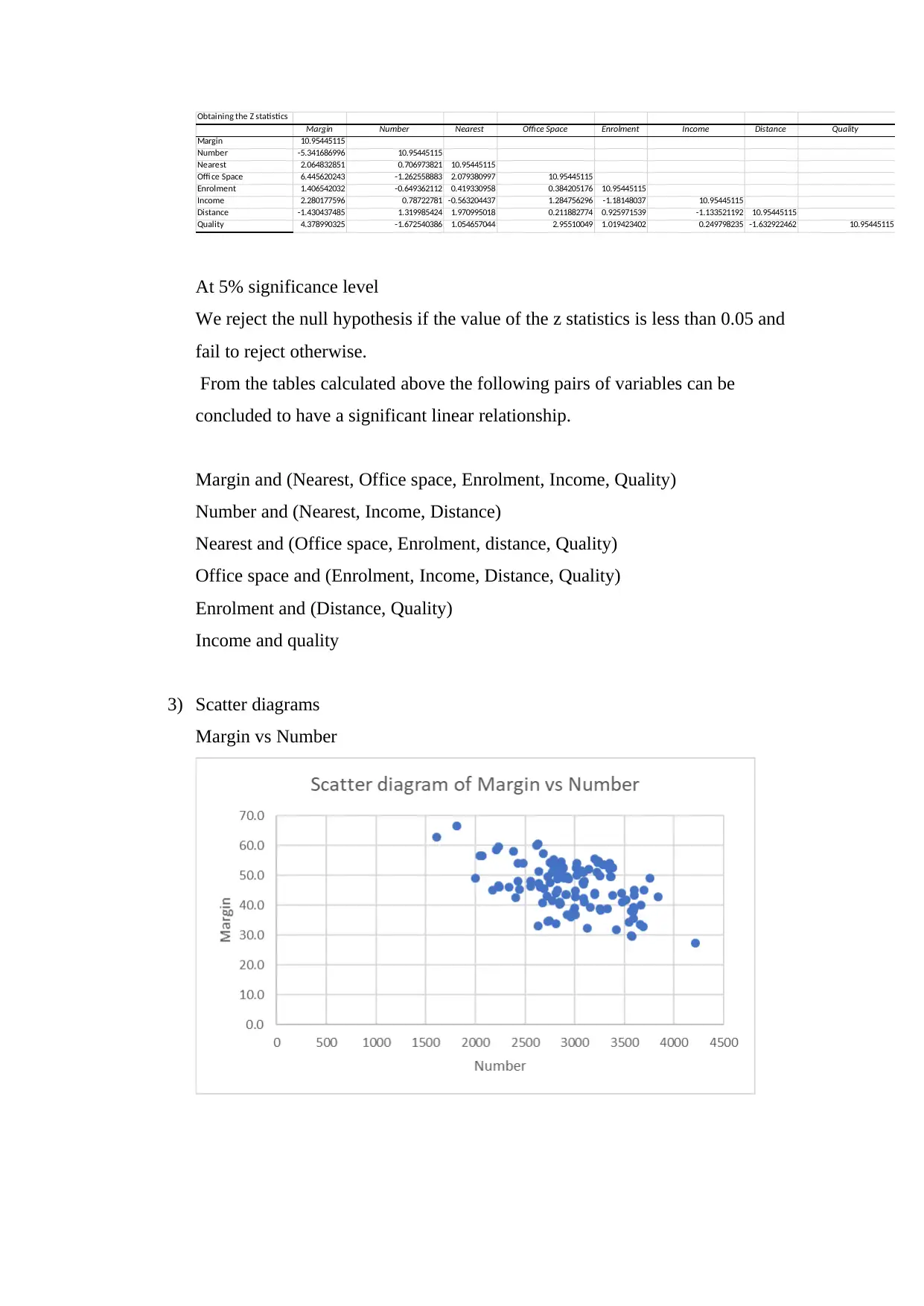
Margin vs Number
Margin Number Nearest Office Space Enrolment Income Distance Quality
Margin 10.95445115
Number -5.341686996 10.95445115
Nearest 2.064832851 0.706973821 10.95445115
Offi ce Space 6.445620243 -1.262558883 2.079380997 10.95445115
Enrolment 1.406542032 -0.649362112 0.419330958 0.384205176 10.95445115
Income 2.280177596 0.78722781 -0.563204437 1.284756296 -1.18148037 10.95445115
Distance -1.430437485 1.319985424 1.970995018 0.211882774 0.925971539 -1.133521192 10.95445115
Quality 4.378990325 -1.672540386 1.054657044 2.95510049 1.019423402 0.249798235 -1.632922462 10.95445115
At 5% significance level
We reject the null hypothesis if the value of the z statistics is less than 0.05 and
fail to reject otherwise.
From the tables calculated above the following pairs of variables can be
concluded to have a significant linear relationship.
Margin and (Nearest, Office space, Enrolment, Income, Quality)
Number and (Nearest, Income, Distance)
Nearest and (Office space, Enrolment, distance, Quality)
Office space and (Enrolment, Income, Distance, Quality)
Enrolment and (Distance, Quality)
Income and quality
3) Scatter diagrams
Margin vs Number
⊘ This is a preview!⊘
Do you want full access?
Subscribe today to unlock all pages.
Trusted by 1+ million students worldwide
The regression coefficient of margin and number of given by -0.4876, when this is
compared against the scatter diagram it can be visualised that the two variables
have a weak negative correlation.
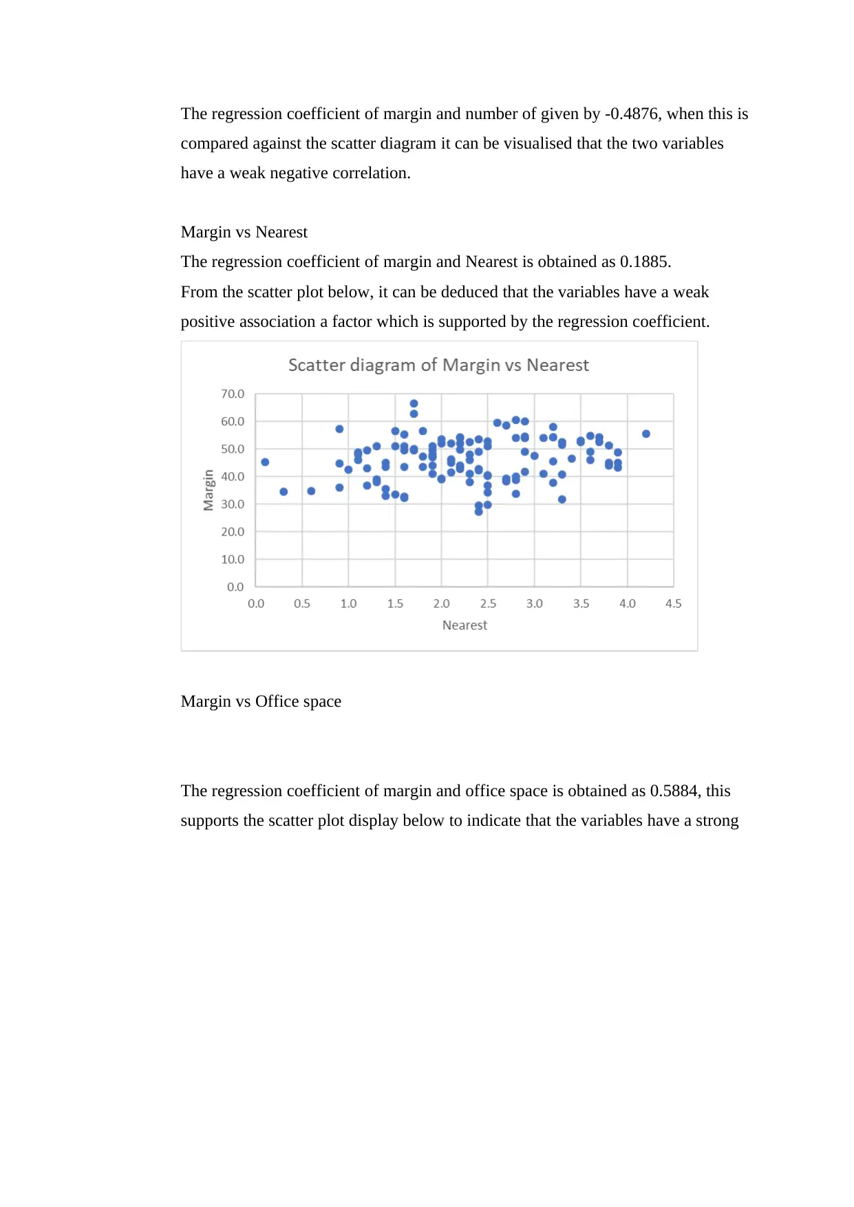
Margin vs Nearest
The regression coefficient of margin and Nearest is obtained as 0.1885.
From the scatter plot below, it can be deduced that the variables have a weak
positive association a factor which is supported by the regression coefficient.
Margin vs Office space
The regression coefficient of margin and office space is obtained as 0.5884, this
supports the scatter plot display below to indicate that the variables have a strong
compared against the scatter diagram it can be visualised that the two variables
have a weak negative correlation.
Margin vs Nearest
The regression coefficient of margin and Nearest is obtained as 0.1885.
From the scatter plot below, it can be deduced that the variables have a weak
positive association a factor which is supported by the regression coefficient.
Margin vs Office space
The regression coefficient of margin and office space is obtained as 0.5884, this
supports the scatter plot display below to indicate that the variables have a strong
Paraphrase This Document
Need a fresh take? Get an instant paraphrase of this document with our AI Paraphraser
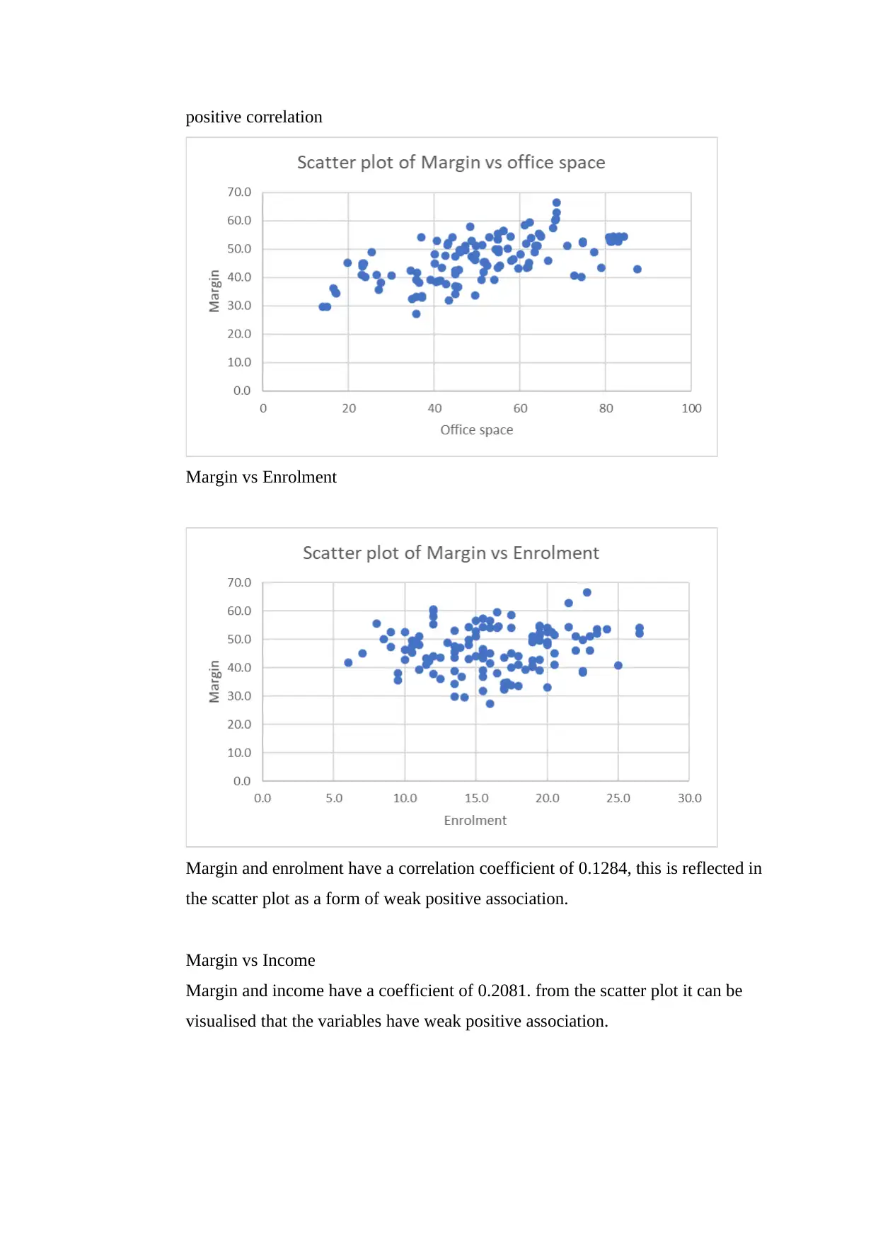
positive correlation
Margin vs Enrolment
Margin and enrolment have a correlation coefficient of 0.1284, this is reflected in
the scatter plot as a form of weak positive association.
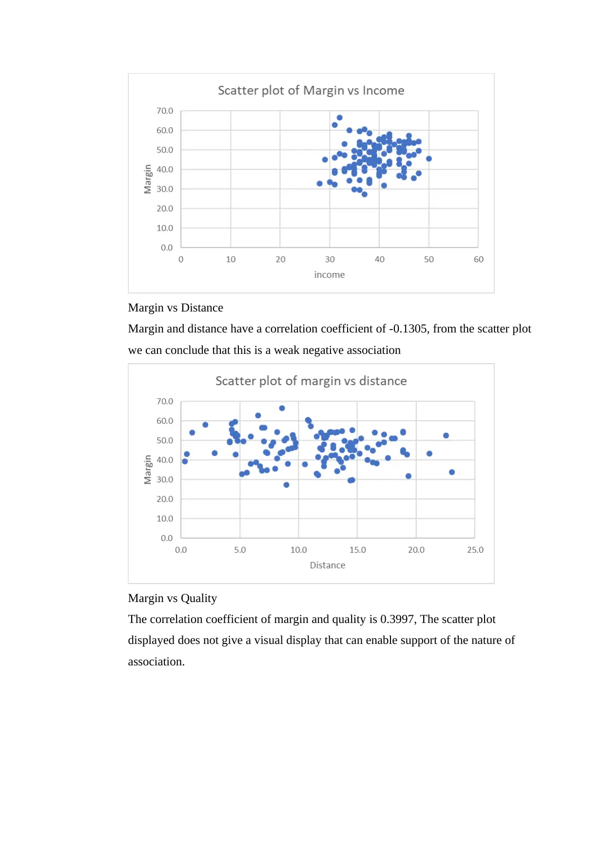
Margin vs Income
Margin and income have a coefficient of 0.2081. from the scatter plot it can be
visualised that the variables have weak positive association.
Margin vs Enrolment
Margin and enrolment have a correlation coefficient of 0.1284, this is reflected in
the scatter plot as a form of weak positive association.
Margin vs Income
Margin and income have a coefficient of 0.2081. from the scatter plot it can be
visualised that the variables have weak positive association.
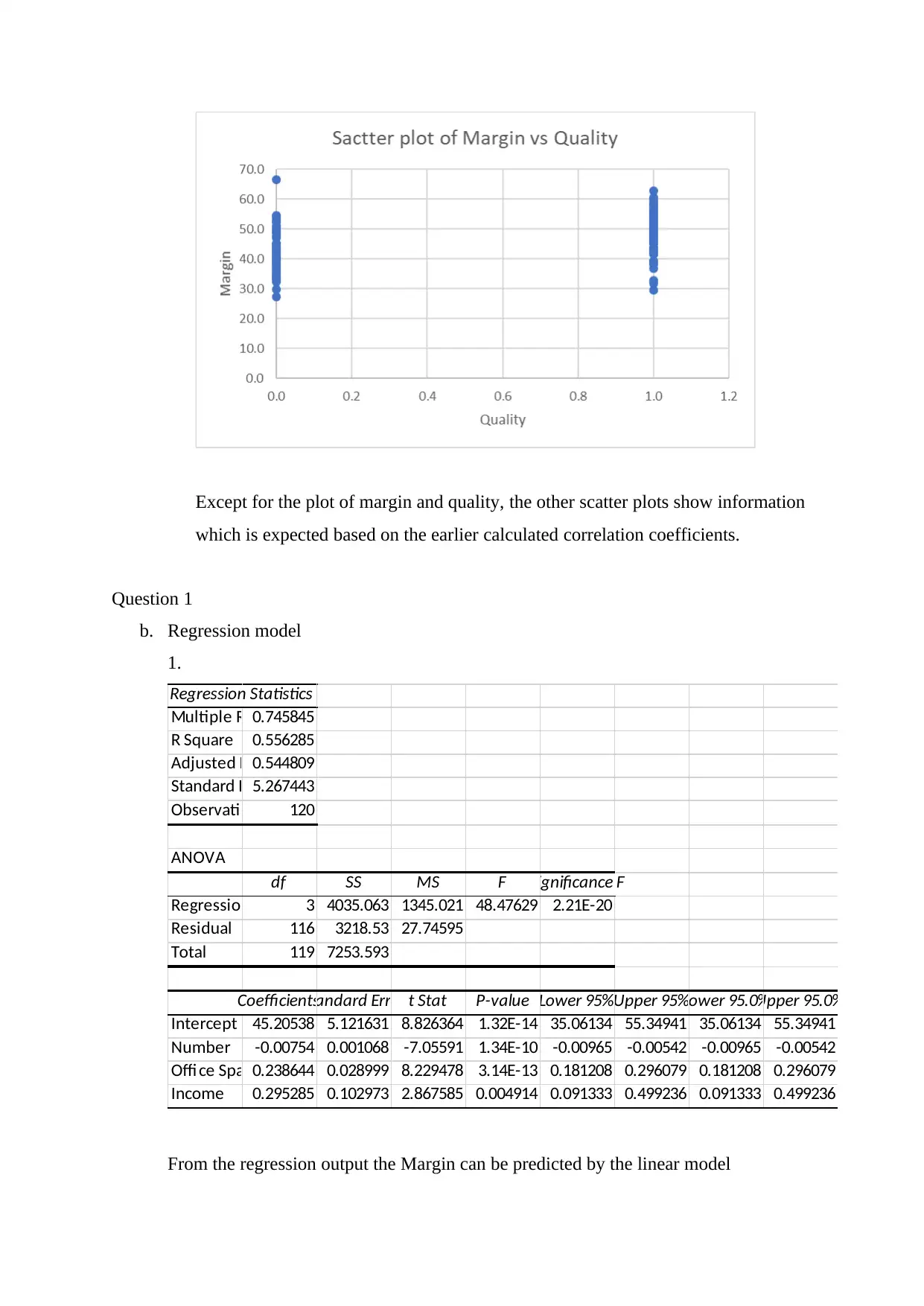
Margin vs Distance
Margin and distance have a correlation coefficient of -0.1305, from the scatter plot
we can conclude that this is a weak negative association
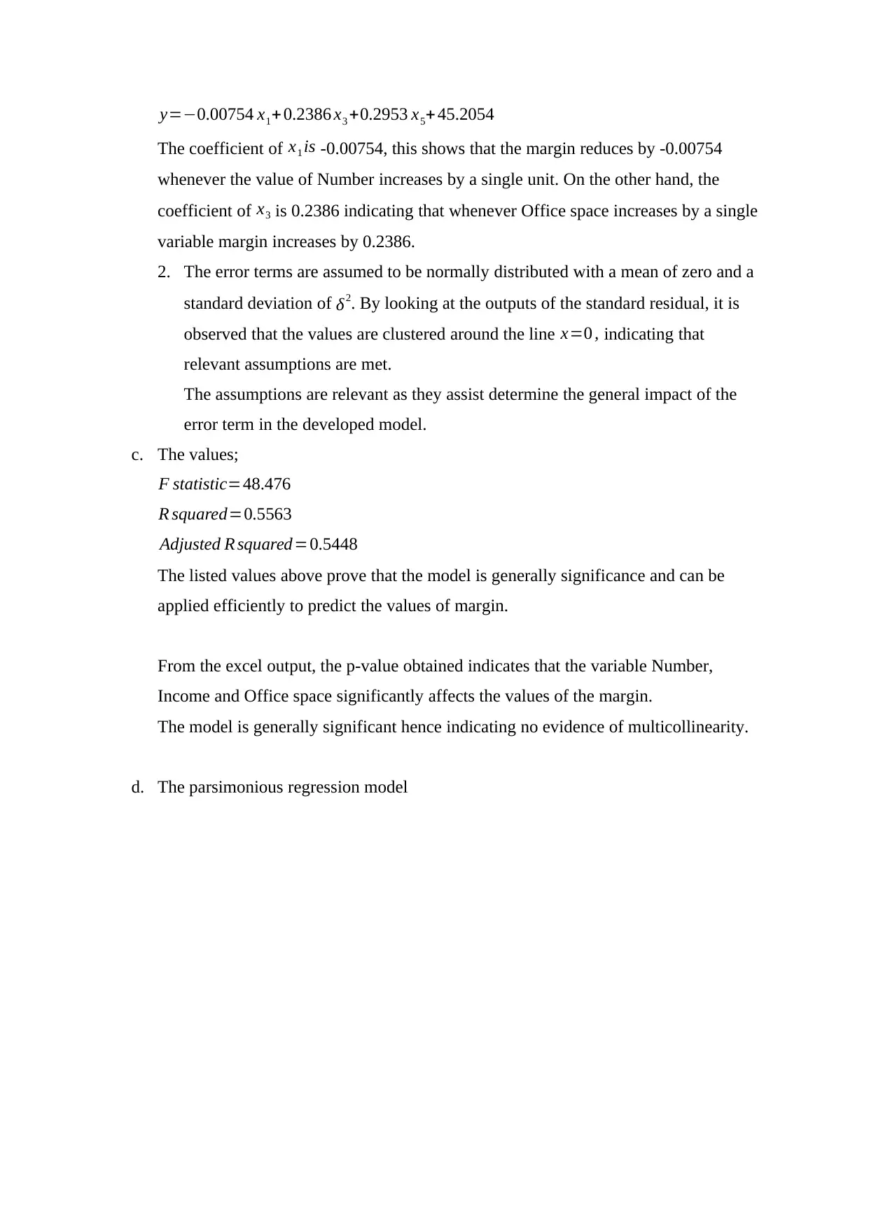
Margin vs Quality
The correlation coefficient of margin and quality is 0.3997, The scatter plot
displayed does not give a visual display that can enable support of the nature of
association.
Margin and distance have a correlation coefficient of -0.1305, from the scatter plot
we can conclude that this is a weak negative association
Margin vs Quality
The correlation coefficient of margin and quality is 0.3997, The scatter plot
displayed does not give a visual display that can enable support of the nature of
association.
⊘ This is a preview!⊘
Do you want full access?
Subscribe today to unlock all pages.
Trusted by 1+ million students worldwide
Except for the plot of margin and quality, the other scatter plots show information
which is expected based on the earlier calculated correlation coefficients.
Question 1
b. Regression model
1.
Regression Statistics
Multiple R 0.745845
R Square 0.556285
Adjusted R Square0.544809
Standard Error5.267443
Observations 120
ANOVA
df SS MS F Significance F
Regression 3 4035.063 1345.021 48.47629 2.21E-20
Residual 116 3218.53 27.74595
Total 119 7253.593
CoefficientsStandard Error t Stat P-value Lower 95%Upper 95%Lower 95.0%Upper 95.0%
Intercept 45.20538 5.121631 8.826364 1.32E-14 35.06134 55.34941 35.06134 55.34941
Number -0.00754 0.001068 -7.05591 1.34E-10 -0.00965 -0.00542 -0.00965 -0.00542
Offi ce Space0.238644 0.028999 8.229478 3.14E-13 0.181208 0.296079 0.181208 0.296079
Income 0.295285 0.102973 2.867585 0.004914 0.091333 0.499236 0.091333 0.499236
From the regression output the Margin can be predicted by the linear model
Paraphrase This Document
Need a fresh take? Get an instant paraphrase of this document with our AI Paraphraser
y=−0.00754 x1+ 0.2386 x3 +0.2953 x5+ 45.2054
The coefficient of x1 is -0.00754, this shows that the margin reduces by -0.00754
whenever the value of Number increases by a single unit. On the other hand, the
coefficient of x3 is 0.2386 indicating that whenever Office space increases by a single
variable margin increases by 0.2386.
2. The error terms are assumed to be normally distributed with a mean of zero and a
standard deviation of δ2. By looking at the outputs of the standard residual, it is
observed that the values are clustered around the line x=0 , indicating that
relevant assumptions are met.
The assumptions are relevant as they assist determine the general impact of the
error term in the developed model.
c. The values;
F statistic=48.476
R squared=0.5563
Adjusted R squared=0.5448
The listed values above prove that the model is generally significance and can be
applied efficiently to predict the values of margin.
From the excel output, the p-value obtained indicates that the variable Number,
Income and Office space significantly affects the values of the margin.
The model is generally significant hence indicating no evidence of multicollinearity.
d. The parsimonious regression model
Regression Statistics
Multiple R 0.788774292
R Square 0.622164884
Adjusted R Square 0.598550189
Standard Error 4.946736161
Observations 120
ANOVA
df SS MS F Significance F
Regression 7 4512.931001 644.7044287 26.34651389 5.09941E-21
Residual 112 2740.662249 24.47019865
Total 119 7253.59325
Coefficients Standard Error t Stat P-value Lower 95% Upper 95% Lower 95.0% Upper 95.0%
Intercept 39.18908567 5.432345495 7.214026743 6.86295E-11 28.42558942 49.95258192 28.42558942 49.95258192
Number -0.007127895 0.001022621 -6.970224269 2.31451E-10 -0.009154086 -0.005101703 -0.009154086 -0.005101703
Nearest 1.214608653 0.550369145 2.206898159 0.029361086 0.124122741 2.305094565 0.124122741 2.305094565
Offi ce Space 0.204264352 0.028711505 7.114372899 1.12996E-10 0.147376186 0.261152519 0.147376186 0.261152519
Enrolment 0.166182752 0.105179027 1.579998952 0.116927236 -0.042216007 0.374581512 -0.042216007 0.374581512
Income 0.315331628 0.09806562 3.215516581 0.001701979 0.121027172 0.509636084 0.121027172 0.509636084
Distance -0.118814121 0.097302304 -1.221082301 0.224619153 -0.311606164 0.073977921 -0.311606164 0.073977921
Quality 2.820949378 0.97252758 2.900636894 0.004483716 0.894010643 4.747888114 0.894010643 4.747888114
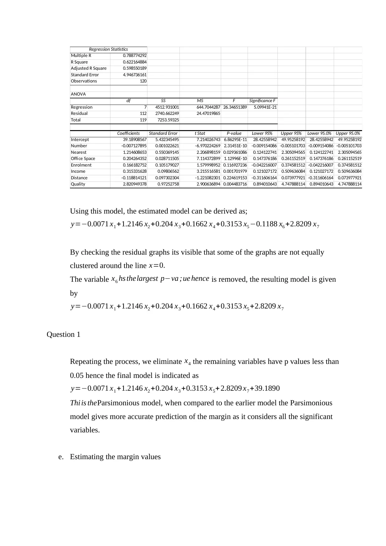
Using this model, the estimated model can be derived as;
y=−0.0071 x1 +1.2146 x2 +0.204 x3 +0.1662 x4 +0.3153 x5 −0.1188 x6 +2.8209 x7
By checking the residual graphs its visible that some of the graphs are not equally
clustered around the line x=0.
The variable x6 hs thelargest p−va ;ue hence is removed, the resulting model is given
by
y=−0.0071 x1 +1.2146 x2 +0.204 x3 +0.1662 x4 +0.3153 x5 +2.8209 x7
Question 1
Repeating the process, we eliminate x4 the remaining variables have p values less than
0.05 hence the final model is indicated as
y=−0.0071 x1 +1.2146 x2 +0.204 x3 +0.3153 x5+ 2.8209 x7 +39.1890
Thi is theParsimonious model, when compared to the earlier model the Parsimonious
model gives more accurate prediction of the margin as it considers all the significant
variables.
e. Estimating the margin values
Multiple R 0.788774292
R Square 0.622164884
Adjusted R Square 0.598550189
Standard Error 4.946736161
Observations 120
ANOVA
df SS MS F Significance F
Regression 7 4512.931001 644.7044287 26.34651389 5.09941E-21
Residual 112 2740.662249 24.47019865
Total 119 7253.59325
Coefficients Standard Error t Stat P-value Lower 95% Upper 95% Lower 95.0% Upper 95.0%
Intercept 39.18908567 5.432345495 7.214026743 6.86295E-11 28.42558942 49.95258192 28.42558942 49.95258192
Number -0.007127895 0.001022621 -6.970224269 2.31451E-10 -0.009154086 -0.005101703 -0.009154086 -0.005101703
Nearest 1.214608653 0.550369145 2.206898159 0.029361086 0.124122741 2.305094565 0.124122741 2.305094565
Offi ce Space 0.204264352 0.028711505 7.114372899 1.12996E-10 0.147376186 0.261152519 0.147376186 0.261152519
Enrolment 0.166182752 0.105179027 1.579998952 0.116927236 -0.042216007 0.374581512 -0.042216007 0.374581512
Income 0.315331628 0.09806562 3.215516581 0.001701979 0.121027172 0.509636084 0.121027172 0.509636084
Distance -0.118814121 0.097302304 -1.221082301 0.224619153 -0.311606164 0.073977921 -0.311606164 0.073977921
Quality 2.820949378 0.97252758 2.900636894 0.004483716 0.894010643 4.747888114 0.894010643 4.747888114
Using this model, the estimated model can be derived as;
y=−0.0071 x1 +1.2146 x2 +0.204 x3 +0.1662 x4 +0.3153 x5 −0.1188 x6 +2.8209 x7
By checking the residual graphs its visible that some of the graphs are not equally
clustered around the line x=0.
The variable x6 hs thelargest p−va ;ue hence is removed, the resulting model is given
by
y=−0.0071 x1 +1.2146 x2 +0.204 x3 +0.1662 x4 +0.3153 x5 +2.8209 x7
Question 1
Repeating the process, we eliminate x4 the remaining variables have p values less than
0.05 hence the final model is indicated as
y=−0.0071 x1 +1.2146 x2 +0.204 x3 +0.3153 x5+ 2.8209 x7 +39.1890
Thi is theParsimonious model, when compared to the earlier model the Parsimonious
model gives more accurate prediction of the margin as it considers all the significant
variables.
e. Estimating the margin values
⊘ This is a preview!⊘
Do you want full access?
Subscribe today to unlock all pages.
Trusted by 1+ million students worldwide
Variables 4 8 19 94
y 31.9 50.2 62.8 34.8
x1 3422 30121 1613 2740
x2 3.3 1.7 1.7 0.6
x3 43.4 57.2 68.6 16.9
x4 15.5 8.5 21.5 17.2
x5 41 45 31 38
x6 19.4 8.8 6.6 7.3
x7 1 0 1 0
original model 41.86606 -154.971 58.56564 39.79954
Parsimonous model 43.50278 -146.748 56.39112 35.89276
The original model makes abetter forecast when compared to the parsimonious model.
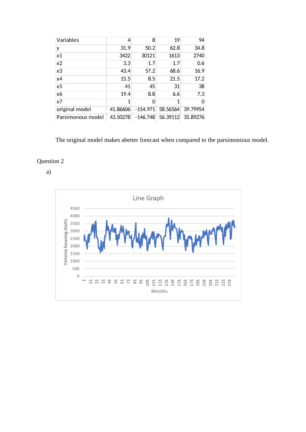
Question 2
a)
y 31.9 50.2 62.8 34.8
x1 3422 30121 1613 2740
x2 3.3 1.7 1.7 0.6
x3 43.4 57.2 68.6 16.9
x4 15.5 8.5 21.5 17.2
x5 41 45 31 38
x6 19.4 8.8 6.6 7.3
x7 1 0 1 0
original model 41.86606 -154.971 58.56564 39.79954
Parsimonous model 43.50278 -146.748 56.39112 35.89276
The original model makes abetter forecast when compared to the parsimonious model.
Question 2
a)
Paraphrase This Document
Need a fresh take? Get an instant paraphrase of this document with our AI Paraphraser
The values of the Victorian housing charts is symmetrically distributed.
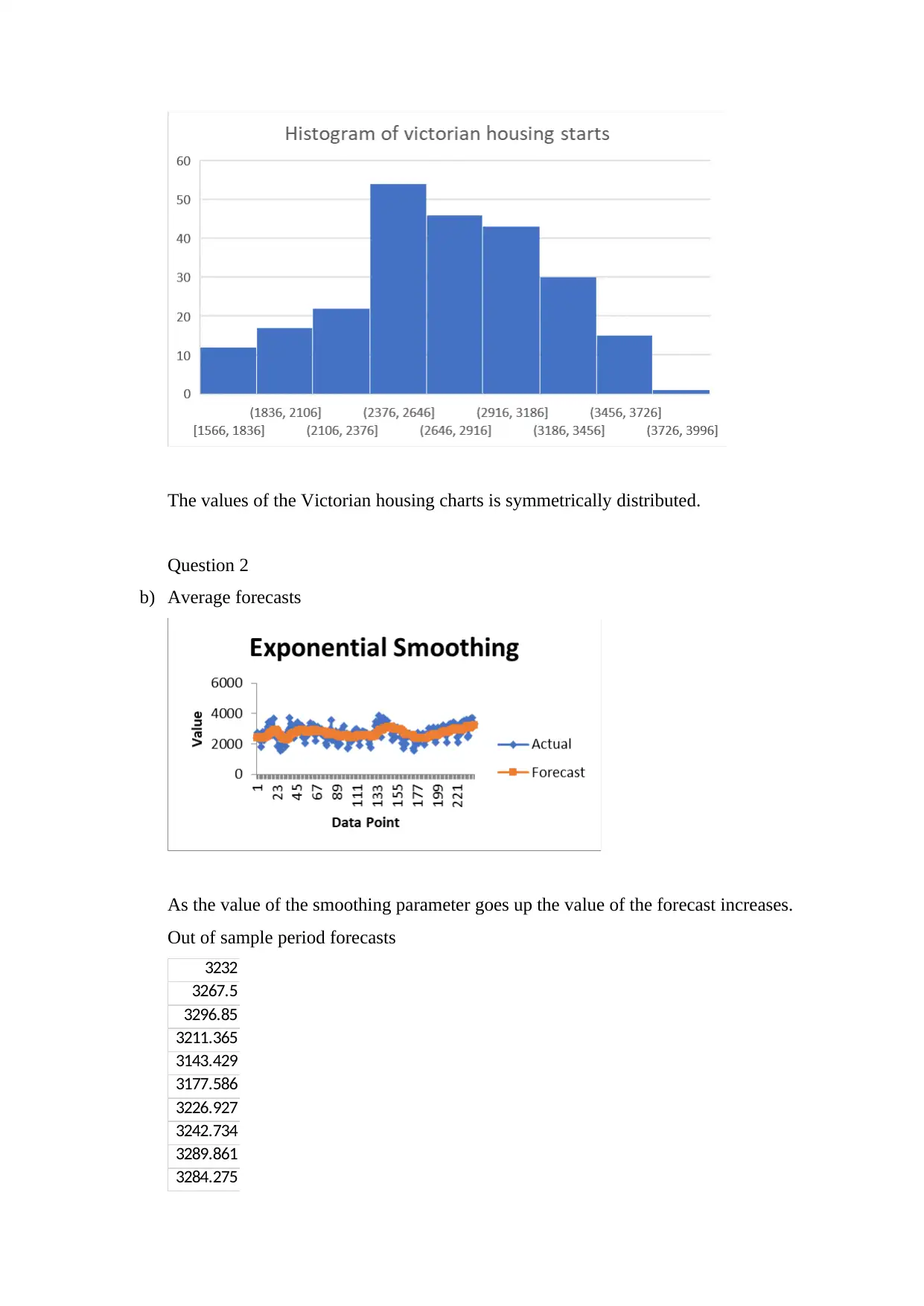
Question 2
b) Average forecasts
As the value of the smoothing parameter goes up the value of the forecast increases.
Out of sample period forecasts
3232
3267.5
3296.85
3211.365
3143.429
3177.586
3226.927
3242.734
3289.861
3284.275
Question 2
b) Average forecasts
As the value of the smoothing parameter goes up the value of the forecast increases.
Out of sample period forecasts
3232
3267.5
3296.85
3211.365
3143.429
3177.586
3226.927
3242.734
3289.861
3284.275
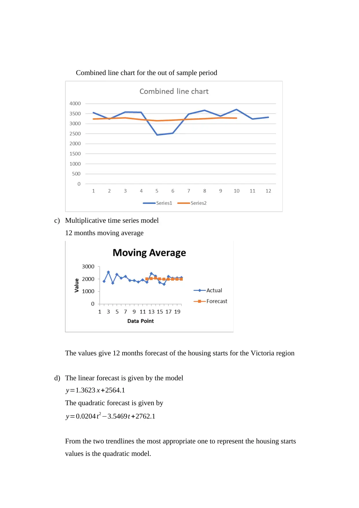
Combined line chart for the out of sample period
c) Multiplicative time series model
12 months moving average
The values give 12 months forecast of the housing starts for the Victoria region
d) The linear forecast is given by the model
y=1.3623 x +2564.1
The quadratic forecast is given by
y=0.0204 t2 −3.5469t +2762.1
From the two trendlines the most appropriate one to represent the housing starts
values is the quadratic model.
⊘ This is a preview!⊘
Do you want full access?
Subscribe today to unlock all pages.
Trusted by 1+ million students worldwide
1 out of 14
Related Documents


Your All-in-One AI-Powered Toolkit for Academic Success.
+13062052269
info@desklib.com
Available 24*7 on WhatsApp / Email
![[object Object]](/_next/static/media/star-bottom.7253800d.svg)
Unlock your academic potential
Copyright © 2020–2026 A2Z Services. All Rights Reserved. Developed and managed by ZUCOL.