Business Decision Making Report: Syngenta's Market Analysis
VerifiedAdded on 2020/02/05
|23
|4708
|76
Report
AI Summary
This report provides a comprehensive analysis of business decision-making processes, focusing on a case study of Syngenta's potential market expansion into the UK. The report encompasses various aspects of data analysis, including the collection of primary and secondary data, the application of survey methodologies, and the use of sampling methods. It delves into the design of market survey questionnaires and the calculation of key statistical measures such as mean, median, mode, standard deviation, and correlation coefficients to interpret market trends and consumer preferences. Furthermore, the report presents visual representations of data through graphs and charts, including sales and profit trend lines, to illustrate business performance. It also incorporates project management tools like Gantt charts and network diagrams to outline project timelines and critical paths. The report concludes with a financial analysis, calculating metrics like Net Present Value (NPV), Average Rate of Return (ARR), and payback period to assess the financial viability of potential projects, providing recommendations based on these findings. The report is a complete guide for business decision making and financial planning.

Business decision making
Paraphrase This Document
Need a fresh take? Get an instant paraphrase of this document with our AI Paraphraser
TABLE OF CONTENTS
Introduction......................................................................................................................................4
Task 1...............................................................................................................................................4
Q.1................................................................................................................................................4
1.1 Planning for collection of primary and secondary data.........................................................4
1.2 Discussing the use of survey methodology and sampling method........................................4
3.4 Preparing a formal report for Director of the Syngenta.........................................................5
Q.2 ...............................................................................................................................................6
1.3 Designing a market survey questionnaire..............................................................................6
Task 2...............................................................................................................................................7
Q.1 ...............................................................................................................................................7
2.1 & 2.2 Calculating mean, median and mode along with their significance............................7
Q.2................................................................................................................................................9
2.3 Calculating range and standard deviation and their significance...........................................9
Q.3 .............................................................................................................................................10
2.4 Explaining the use of Quartile, Percentiles and the Correlation coefficient........................10
Task 3.............................................................................................................................................11
Q.1 .............................................................................................................................................11
3.1 Preparing different graphs along with their conclusions.....................................................11
Q.2 .............................................................................................................................................13
3.2 Producing sales and profit line graphs showing trend lines.................................................13
Q.3 Preparing a presentation......................................................................................................14
Task 4.............................................................................................................................................14
Q.1..............................................................................................................................................14
4.1 Preparing a Gantt chart along with their benefits................................................................14
Q.2..............................................................................................................................................16
4.2 Preparing a network diagram...............................................................................................16
Q.3..............................................................................................................................................17
4.3 Calculation of NPV, ARR & pay back period with recommendation ................................17
Conclusion.....................................................................................................................................20
References......................................................................................................................................21
2
Illustration Index
Illustration 1: Column graph of sales.............................................................................................11
Illustration 2: Line graph of profits................................................................................................12
Illustration 3: Bar graph of cost.....................................................................................................13
Illustration 4: Trend line graph of sales and profit........................................................................14
Illustration 5: Gantt chart...............................................................................................................15
Illustration 6: Critical path.............................................................................................................16
Index of Tables
Table 1: Sample frame.....................................................................................................................5
Table 2: Preparing a Report.............................................................................................................5
Table 3: Grouped data......................................................................................................................7
Table 4: Calculation of Mean..........................................................................................................7
Table 5: Calculation of Median.......................................................................................................8
Table 6: Calculation of Mode..........................................................................................................8
Table 7: Calculation of Standard deviation.....................................................................................9
Table 8: Values of Quartile............................................................................................................10
Table 9: Values of Percentile.........................................................................................................10
Table 10: Values of correlation coefficient...................................................................................11
Table 11: Last 10 years values of sales, profit and cost.................................................................11
Table 12: 2 projects Grangemouth and Inverness..........................................................................17
Table 13: Calculation of Net present value for project Grangemouth...........................................17
Table 14: Calculation of Net present value for project Inverness.................................................17
Table 15: Calculation of average rate of return for project Grangemouth....................................18
Table 16: Calculation of average rate of return for project Inverness...........................................18
Table 17: Calculation of Pay back period for Project Grangemouth.............................................19
Table 18: Calculation of Pay back period for Project Inverness...................................................19
Table 19: Calculation of Internal rate of return for project Grangemouth....................................19
Table 20: Calculation of Internal rate of return for project Inverness...........................................20
3
⊘ This is a preview!⊘
Do you want full access?
Subscribe today to unlock all pages.
Trusted by 1+ million students worldwide
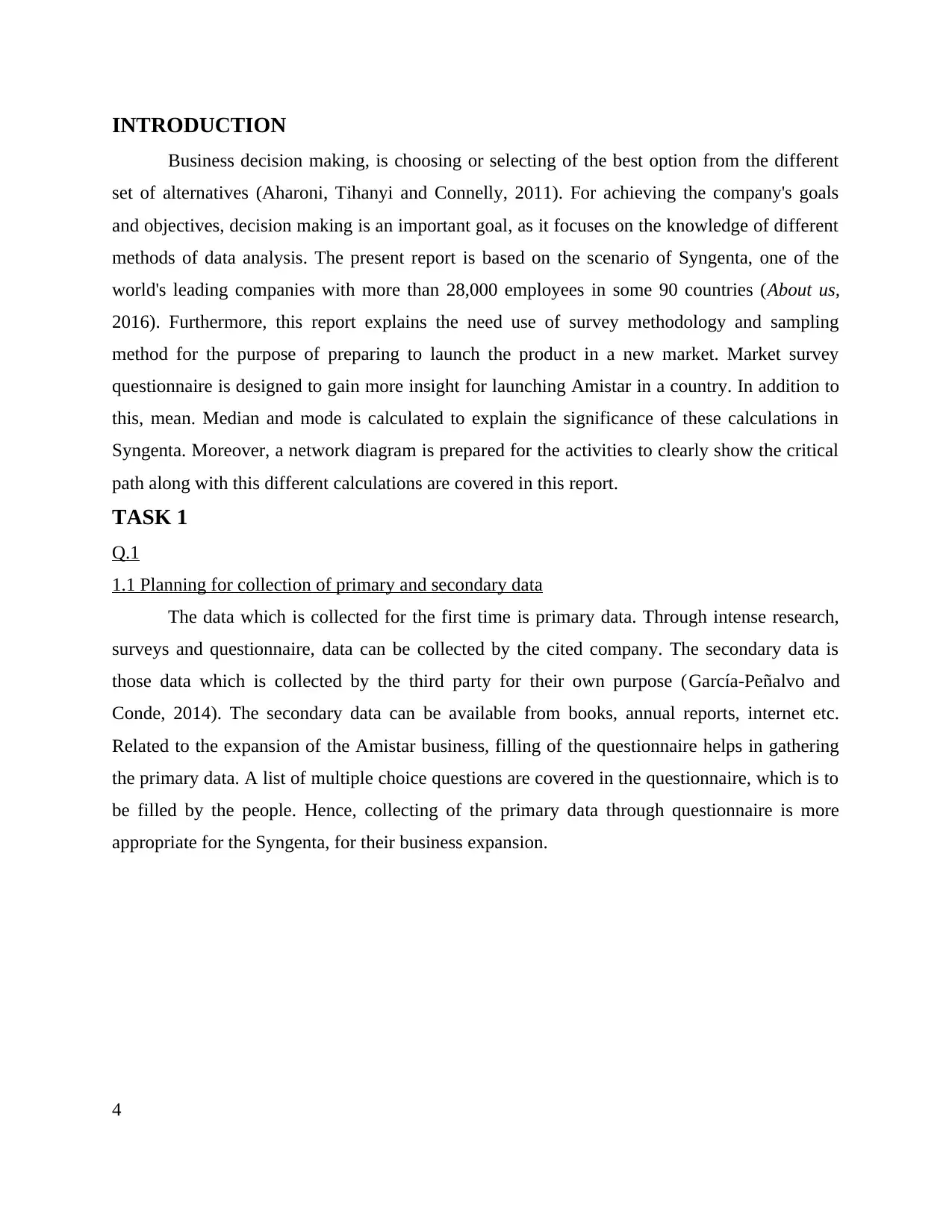
INTRODUCTION
Business decision making, is choosing or selecting of the best option from the different
set of alternatives (Aharoni, Tihanyi and Connelly, 2011). For achieving the company's goals
and objectives, decision making is an important goal, as it focuses on the knowledge of different
methods of data analysis. The present report is based on the scenario of Syngenta, one of the
world's leading companies with more than 28,000 employees in some 90 countries (About us,
2016). Furthermore, this report explains the need use of survey methodology and sampling
method for the purpose of preparing to launch the product in a new market. Market survey
questionnaire is designed to gain more insight for launching Amistar in a country. In addition to
this, mean. Median and mode is calculated to explain the significance of these calculations in
Syngenta. Moreover, a network diagram is prepared for the activities to clearly show the critical
path along with this different calculations are covered in this report.
TASK 1
Q.1
1.1 Planning for collection of primary and secondary data
The data which is collected for the first time is primary data. Through intense research,
surveys and questionnaire, data can be collected by the cited company. The secondary data is
those data which is collected by the third party for their own purpose (García-Peñalvo and
Conde, 2014). The secondary data can be available from books, annual reports, internet etc.
Related to the expansion of the Amistar business, filling of the questionnaire helps in gathering
the primary data. A list of multiple choice questions are covered in the questionnaire, which is to
be filled by the people. Hence, collecting of the primary data through questionnaire is more
appropriate for the Syngenta, for their business expansion.
4
Paraphrase This Document
Need a fresh take? Get an instant paraphrase of this document with our AI Paraphraser
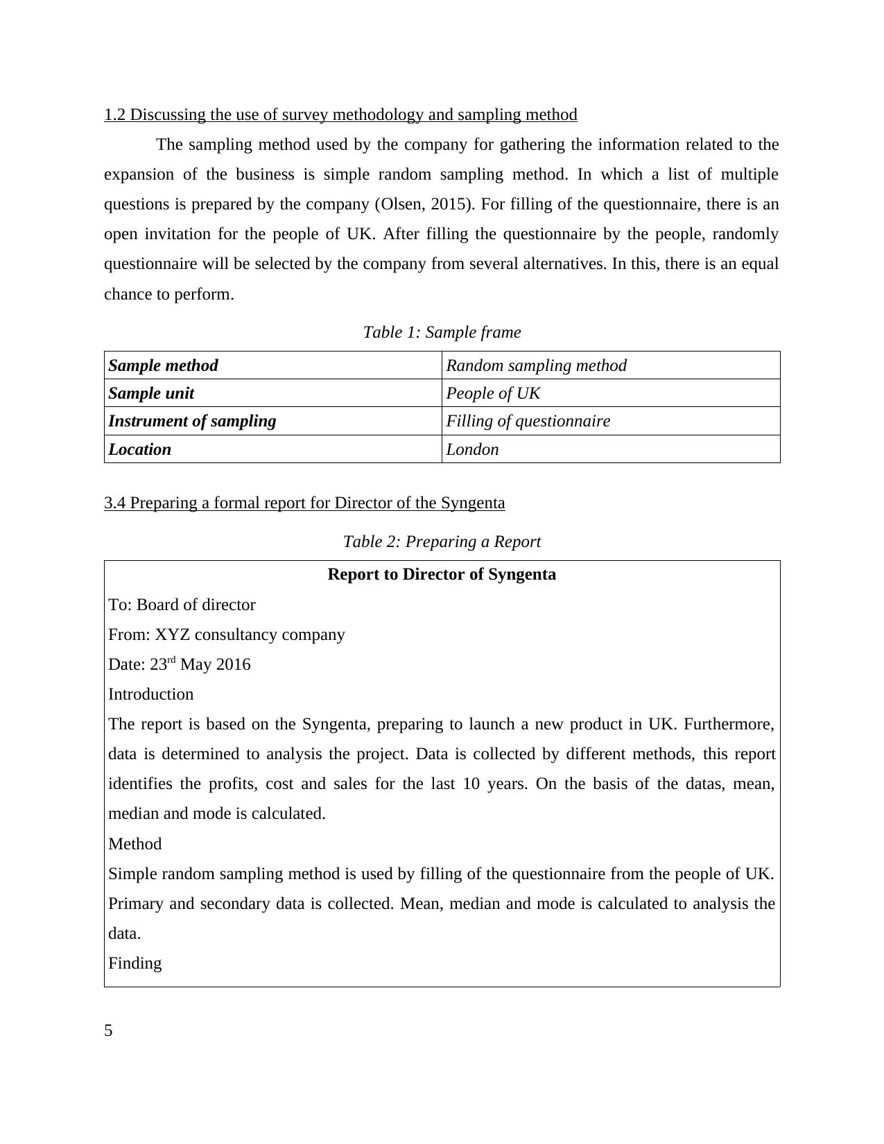
1.2 Discussing the use of survey methodology and sampling method
The sampling method used by the company for gathering the information related to the
expansion of the business is simple random sampling method. In which a list of multiple
questions is prepared by the company (Olsen, 2015). For filling of the questionnaire, there is an
open invitation for the people of UK. After filling the questionnaire by the people, randomly
questionnaire will be selected by the company from several alternatives. In this, there is an equal
chance to perform.
Table 1: Sample frame
Sample method Random sampling method
Sample unit People of UK
Instrument of sampling Filling of questionnaire
Location London
3.4 Preparing a formal report for Director of the Syngenta
Table 2: Preparing a Report
Report to Director of Syngenta
To: Board of director
From: XYZ consultancy company
Date: 23rd May 2016
Introduction
The report is based on the Syngenta, preparing to launch a new product in UK. Furthermore,
data is determined to analysis the project. Data is collected by different methods, this report
identifies the profits, cost and sales for the last 10 years. On the basis of the datas, mean,
median and mode is calculated.
Method
Simple random sampling method is used by filling of the questionnaire from the people of UK.
Primary and secondary data is collected. Mean, median and mode is calculated to analysis the
data.
Finding
5
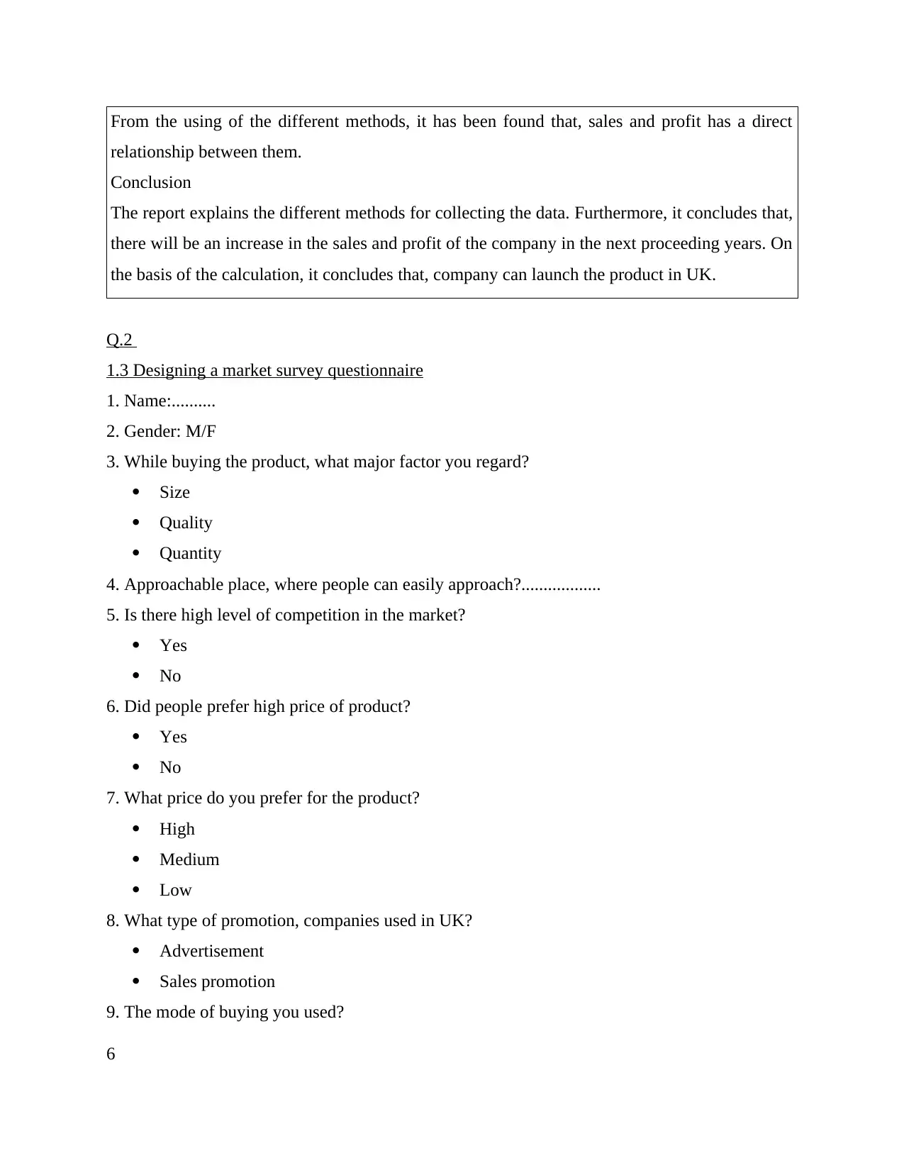
From the using of the different methods, it has been found that, sales and profit has a direct
relationship between them.
Conclusion
The report explains the different methods for collecting the data. Furthermore, it concludes that,
there will be an increase in the sales and profit of the company in the next proceeding years. On
the basis of the calculation, it concludes that, company can launch the product in UK.
Q.2
1.3 Designing a market survey questionnaire
1. Name:..........
2. Gender: M/F
3. While buying the product, what major factor you regard?
Size
Quality
Quantity
4. Approachable place, where people can easily approach?..................
5. Is there high level of competition in the market?
Yes
No
6. Did people prefer high price of product?
Yes
No
7. What price do you prefer for the product?
High
Medium
Low
8. What type of promotion, companies used in UK?
Advertisement
Sales promotion
9. The mode of buying you used?
6
⊘ This is a preview!⊘
Do you want full access?
Subscribe today to unlock all pages.
Trusted by 1+ million students worldwide
Brand stores
Retail shops
Online
10. The business in UK, is beneficial?
Yes
No
11. Kindly give recommendation for launching of Amistar in UK? …..............
TASK 2
Q.1
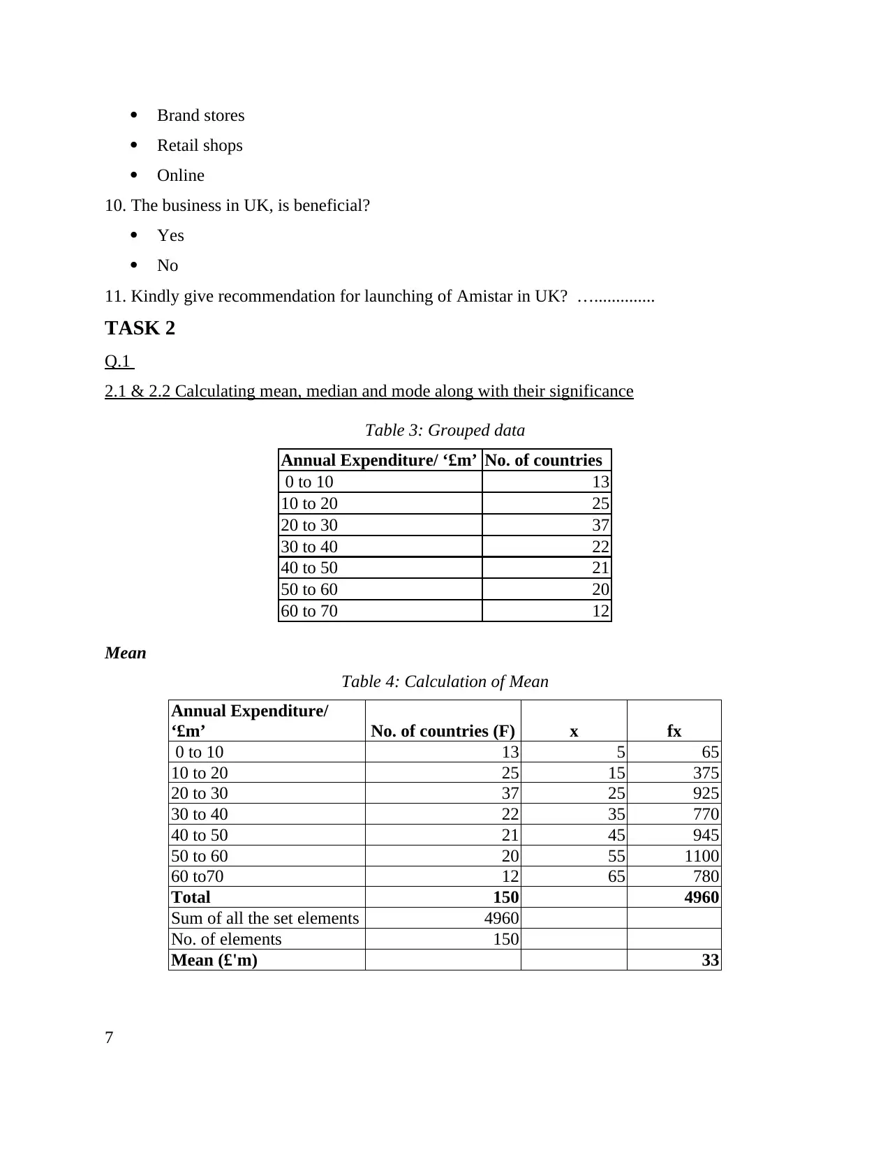
2.1 & 2.2 Calculating mean, median and mode along with their significance
Table 3: Grouped data
Annual Expenditure/ ‘£m’ No. of countries
0 to 10 13
10 to 20 25
20 to 30 37
30 to 40 22
40 to 50 21
50 to 60 20
60 to 70 12
Mean
Table 4: Calculation of Mean
Annual Expenditure/
‘£m’ No. of countries (F) x fx
0 to 10 13 5 65
10 to 20 25 15 375
20 to 30 37 25 925
30 to 40 22 35 770
40 to 50 21 45 945
50 to 60 20 55 1100
60 to70 12 65 780
Total 150 4960
Sum of all the set elements 4960
No. of elements 150
Mean (£'m) 33
7
Retail shops
Online
10. The business in UK, is beneficial?
Yes
No
11. Kindly give recommendation for launching of Amistar in UK? …..............
TASK 2
Q.1
2.1 & 2.2 Calculating mean, median and mode along with their significance
Table 3: Grouped data
Annual Expenditure/ ‘£m’ No. of countries
0 to 10 13
10 to 20 25
20 to 30 37
30 to 40 22
40 to 50 21
50 to 60 20
60 to 70 12
Mean
Table 4: Calculation of Mean
Annual Expenditure/
‘£m’ No. of countries (F) x fx
0 to 10 13 5 65
10 to 20 25 15 375
20 to 30 37 25 925
30 to 40 22 35 770
40 to 50 21 45 945
50 to 60 20 55 1100
60 to70 12 65 780
Total 150 4960
Sum of all the set elements 4960
No. of elements 150
Mean (£'m) 33
7
Paraphrase This Document
Need a fresh take? Get an instant paraphrase of this document with our AI Paraphraser
Mean = Sum of all the set elements / Number of elements
The first measure of central tendency is mean (Smyth and Lecoeuvre, 2015). The mean
value of the country's annual expenditure is the average of the total expenditure of the countries
divided by the number of countries. The mean value is £33, this gives an indication of the total
expenditure in the different countries.
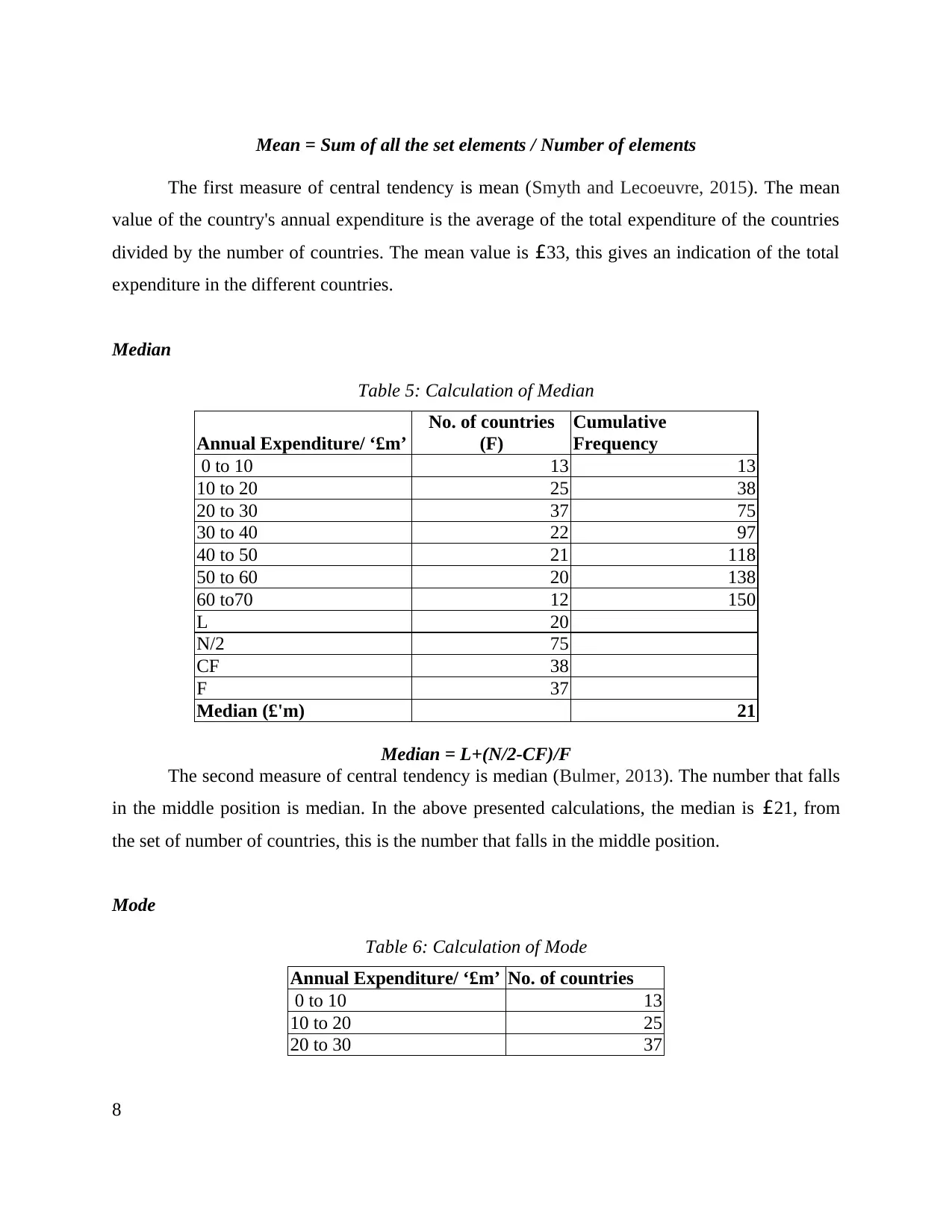
Median
Table 5: Calculation of Median
Annual Expenditure/ ‘£m’
No. of countries
(F)
Cumulative
Frequency
0 to 10 13 13
10 to 20 25 38
20 to 30 37 75
30 to 40 22 97
40 to 50 21 118
50 to 60 20 138
60 to70 12 150
L 20
N/2 75
CF 38
F 37
Median (£'m) 21
Median = L+(N/2-CF)/F
The second measure of central tendency is median (Bulmer, 2013). The number that falls
in the middle position is median. In the above presented calculations, the median is £21, from
the set of number of countries, this is the number that falls in the middle position.
Mode
Table 6: Calculation of Mode
Annual Expenditure/ ‘£m’ No. of countries
0 to 10 13
10 to 20 25
20 to 30 37
8
The first measure of central tendency is mean (Smyth and Lecoeuvre, 2015). The mean
value of the country's annual expenditure is the average of the total expenditure of the countries
divided by the number of countries. The mean value is £33, this gives an indication of the total
expenditure in the different countries.
Median
Table 5: Calculation of Median
Annual Expenditure/ ‘£m’
No. of countries
(F)
Cumulative
Frequency
0 to 10 13 13
10 to 20 25 38
20 to 30 37 75
30 to 40 22 97
40 to 50 21 118
50 to 60 20 138
60 to70 12 150
L 20
N/2 75
CF 38
F 37
Median (£'m) 21
Median = L+(N/2-CF)/F
The second measure of central tendency is median (Bulmer, 2013). The number that falls
in the middle position is median. In the above presented calculations, the median is £21, from
the set of number of countries, this is the number that falls in the middle position.
Mode
Table 6: Calculation of Mode
Annual Expenditure/ ‘£m’ No. of countries
0 to 10 13
10 to 20 25
20 to 30 37
8
30 to 40 22
40 to 50 21
50 to 60 20
60 to70 12
F0 25
F1 37
F3 22
L 20
Mode= L+{(F1-F0)/2F1-
F0-F2}
Mode 20
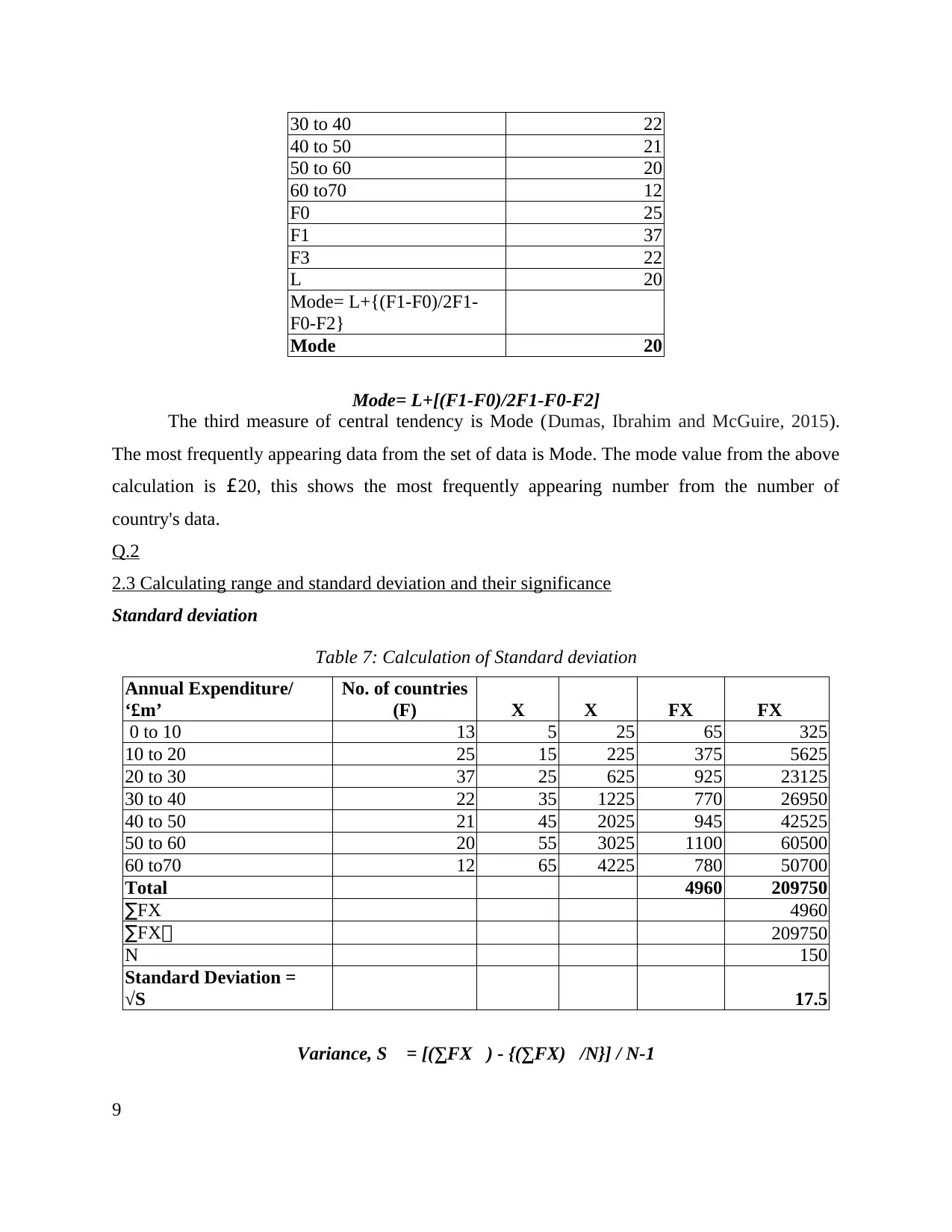
Mode= L+[(F1-F0)/2F1-F0-F2]
The third measure of central tendency is Mode (Dumas, Ibrahim and McGuire, 2015).
The most frequently appearing data from the set of data is Mode. The mode value from the above
calculation is £20, this shows the most frequently appearing number from the number of
country's data.
Q.2
2.3 Calculating range and standard deviation and their significance
Standard deviation
Table 7: Calculation of Standard deviation
Annual Expenditure/
‘£m’
No. of countries
(F) X X FX FX
0 to 10 13 5 25 65 325
10 to 20 25 15 225 375 5625
20 to 30 37 25 625 925 23125
30 to 40 22 35 1225 770 26950
40 to 50 21 45 2025 945 42525
50 to 60 20 55 3025 1100 60500
60 to70 12 65 4225 780 50700
Total 4960 209750
∑FX 4960
∑FX 209750
N 150
Standard Deviation =
√S 17.5
Variance, S = [(∑FX) - {(∑FX)/N}] / N-1
9
40 to 50 21
50 to 60 20
60 to70 12
F0 25
F1 37
F3 22
L 20
Mode= L+{(F1-F0)/2F1-
F0-F2}
Mode 20
Mode= L+[(F1-F0)/2F1-F0-F2]
The third measure of central tendency is Mode (Dumas, Ibrahim and McGuire, 2015).
The most frequently appearing data from the set of data is Mode. The mode value from the above
calculation is £20, this shows the most frequently appearing number from the number of
country's data.
Q.2
2.3 Calculating range and standard deviation and their significance
Standard deviation
Table 7: Calculation of Standard deviation
Annual Expenditure/
‘£m’
No. of countries
(F) X X FX FX
0 to 10 13 5 25 65 325
10 to 20 25 15 225 375 5625
20 to 30 37 25 625 925 23125
30 to 40 22 35 1225 770 26950
40 to 50 21 45 2025 945 42525
50 to 60 20 55 3025 1100 60500
60 to70 12 65 4225 780 50700
Total 4960 209750
∑FX 4960
∑FX 209750
N 150
Standard Deviation =
√S 17.5
Variance, S = [(∑FX) - {(∑FX)/N}] / N-1
9
⊘ This is a preview!⊘
Do you want full access?
Subscribe today to unlock all pages.
Trusted by 1+ million students worldwide
Standard deviation = √S
Standard deviation is the square root of the variance (Ghattas, Soffer and Peleg, 2014). It
is calculated to measure the investment volatility. It gives an indication whether the data is
highly spread or are bunched up closely. From the above calculation, the Standard deviation is
£17.5, which means that the annual expenditure of the countries are closely bunched up.
Range
Range is the differences of the upper class boundary of the highest class and the lowest
class boundary of the lowest class (Powell, Vidgen and Sims, 2015). As, this shows the boundary
of the class hence, it is calculated so to understand how annual expenditure in different countries
are spread out. From the above presented data, the range of the annual expenditure is 70.
Q.3
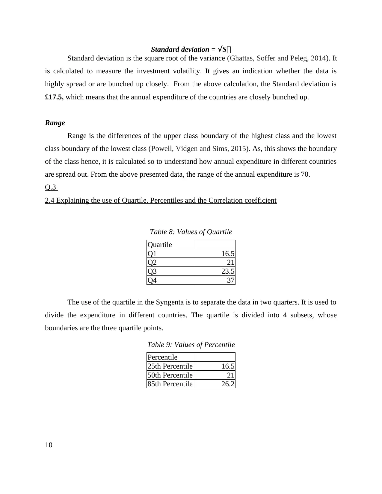
2.4 Explaining the use of Quartile, Percentiles and the Correlation coefficient
Table 8: Values of Quartile
Quartile
Q1 16.5
Q2 21
Q3 23.5
Q4 37
The use of the quartile in the Syngenta is to separate the data in two quarters. It is used to
divide the expenditure in different countries. The quartile is divided into 4 subsets, whose
boundaries are the three quartile points.
Table 9: Values of Percentile
Percentile
25th Percentile 16.5
50th Percentile 21
85th Percentile 26.2
10
Standard deviation is the square root of the variance (Ghattas, Soffer and Peleg, 2014). It
is calculated to measure the investment volatility. It gives an indication whether the data is
highly spread or are bunched up closely. From the above calculation, the Standard deviation is
£17.5, which means that the annual expenditure of the countries are closely bunched up.
Range
Range is the differences of the upper class boundary of the highest class and the lowest
class boundary of the lowest class (Powell, Vidgen and Sims, 2015). As, this shows the boundary
of the class hence, it is calculated so to understand how annual expenditure in different countries
are spread out. From the above presented data, the range of the annual expenditure is 70.
Q.3
2.4 Explaining the use of Quartile, Percentiles and the Correlation coefficient
Table 8: Values of Quartile
Quartile
Q1 16.5
Q2 21
Q3 23.5
Q4 37
The use of the quartile in the Syngenta is to separate the data in two quarters. It is used to
divide the expenditure in different countries. The quartile is divided into 4 subsets, whose
boundaries are the three quartile points.
Table 9: Values of Percentile
Percentile
25th Percentile 16.5
50th Percentile 21
85th Percentile 26.2
10
Paraphrase This Document
Need a fresh take? Get an instant paraphrase of this document with our AI Paraphraser
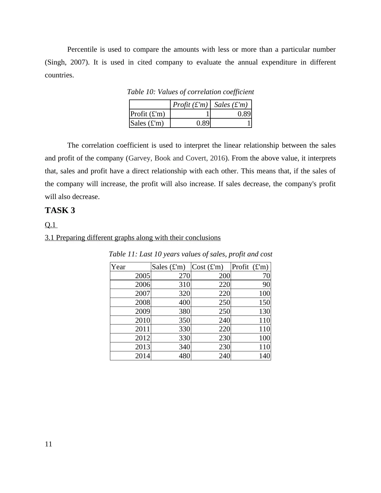
Percentile is used to compare the amounts with less or more than a particular number
(Singh, 2007). It is used in cited company to evaluate the annual expenditure in different
countries.
Table 10: Values of correlation coefficient
Profit (£'m) Sales (£'m)
Profit (£'m) 1 0.89
Sales (£'m) 0.89 1
The correlation coefficient is used to interpret the linear relationship between the sales
and profit of the company (Garvey, Book and Covert, 2016). From the above value, it interprets
that, sales and profit have a direct relationship with each other. This means that, if the sales of
the company will increase, the profit will also increase. If sales decrease, the company's profit
will also decrease.
TASK 3
Q.1
3.1 Preparing different graphs along with their conclusions
Table 11: Last 10 years values of sales, profit and cost
Year Sales (£'m) Cost (£'m) Profit (£'m)
2005 270 200 70
2006 310 220 90
2007 320 220 100
2008 400 250 150
2009 380 250 130
2010 350 240 110
2011 330 220 110
2012 330 230 100
2013 340 230 110
2014 480 240 140
11
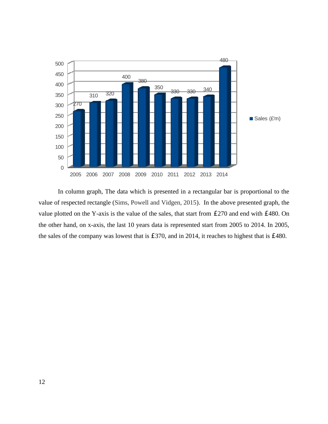
In column graph, The data which is presented in a rectangular bar is proportional to the
value of respected rectangle (Sims, Powell and Vidgen, 2015). In the above presented graph, the
value plotted on the Y-axis is the value of the sales, that start from £270 and end with £480. On
the other hand, on x-axis, the last 10 years data is represented start from 2005 to 2014. In 2005,
the sales of the company was lowest that is £370, and in 2014, it reaches to highest that is £480.
12
2005 2006 2007 2008 2009 2010 2011 2012 2013 2014
0
50
100
150
200
250
300
350
400
450
500
270
310 320
400 380
350 330 330 340
480
Sales (£'m)
⊘ This is a preview!⊘
Do you want full access?
Subscribe today to unlock all pages.
Trusted by 1+ million students worldwide
1 out of 23
Related Documents


Your All-in-One AI-Powered Toolkit for Academic Success.
+13062052269
info@desklib.com
Available 24*7 on WhatsApp / Email
![[object Object]](/_next/static/media/star-bottom.7253800d.svg)
Unlock your academic potential
Copyright © 2020–2026 A2Z Services. All Rights Reserved. Developed and managed by ZUCOL.