Modeling and Simulation of a DC Motor: ELEC431 Project, University

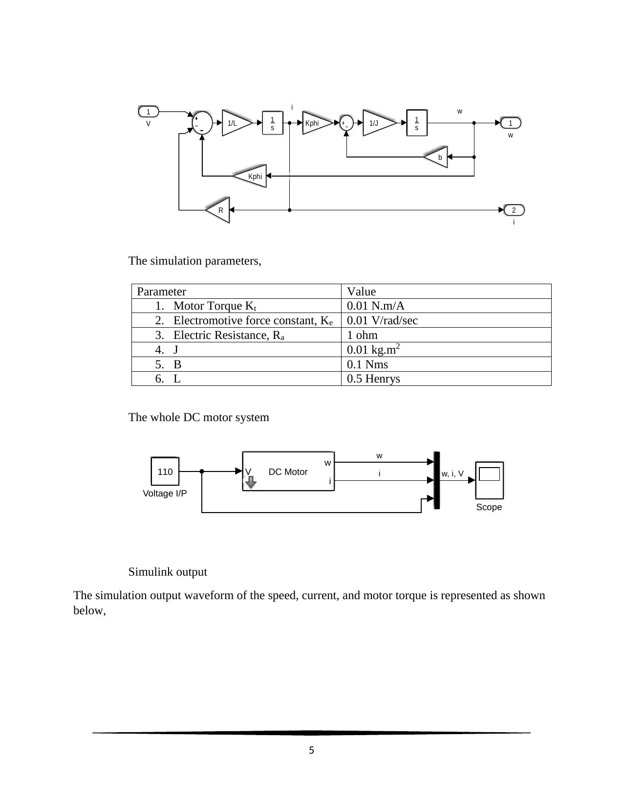
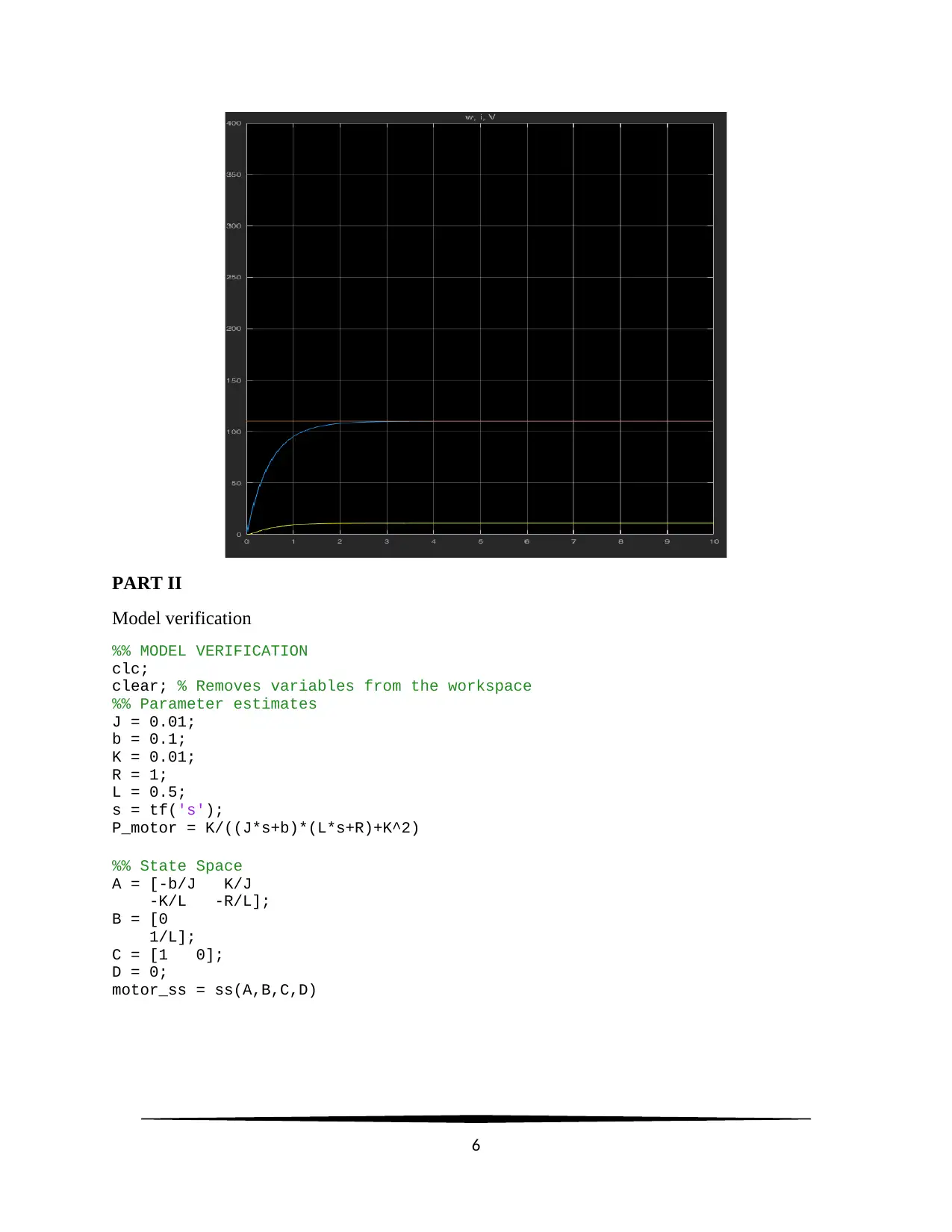
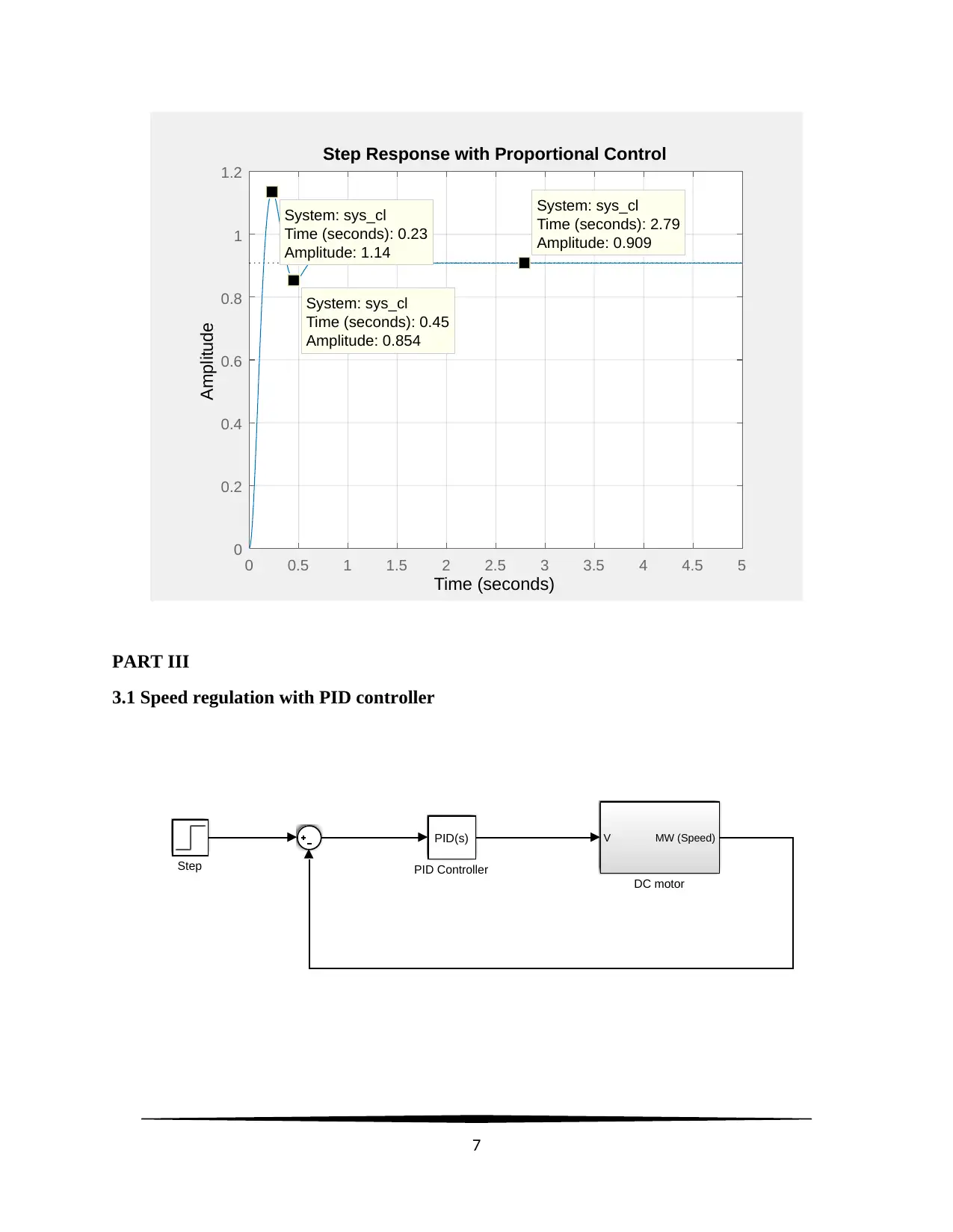
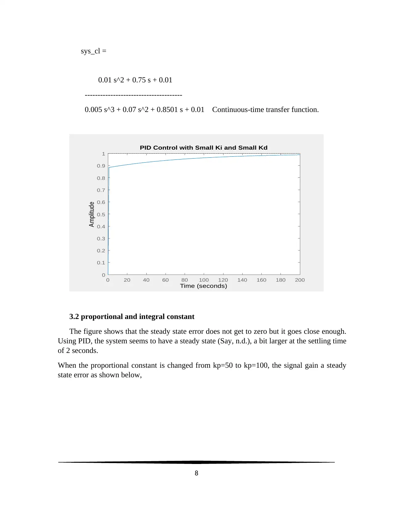
This project report details the modeling and simulation of a DC motor using Simulink and MATLAB. The assignment begins with an introduction to DC motors, their applications, and operational principles. It then presents a Simulink model of the DC motor system, including subsystem diagrams and simulation parameters, followed by the results and observations of the simulation output for speed, current, and motor torque. The report includes a model verification section with MATLAB code for parameter estimation and state-space representation. Furthermore, it explores speed regulation using a PID controller, analyzing the effects of proportional, integral, and derivative constants on system performance, including steady-state error, rise time, overshoot, and settling time. The discussion section summarizes the findings, highlighting the challenges encountered, such as steady-state errors, and the solutions implemented, such as introducing a reference unity feedback and using a derivative component to achieve a smooth output signal. The report concludes with a list of references.

UNIVERSITY AFFILIATION
ELEC431
SOFTWARE ENGINEERING AND PROGRAMMING
ASSIGNMENT 2
MODELLING AND SIMULATION OF A DC MOTOR
STUDENT NAME
STUDENT ID
PROFESSOR (tutor)
DATE OF SUBMISSION
1

TABLE OF CONTENTS
INTRODUCTION.......................................................................................................................................2
RESULTS AND OBSERVATION.............................................................................................................4
DISCUSSION.............................................................................................................................................9
REFERENCES..........................................................................................................................................10
2

INTRODUCTION
DC motors are quite rare in the implementation of engineering applications. There are many
ways in which the DC motors are applied especially in the automotive and electrical field. The
DC motor speed can be controlled over a very wide range. The DC machines are quite similar to
the AC machines. The DC motors have a DC output as they convert the AC components to DC
using the commutator. As such, the electromagnetic energy becomes motion. They use the
batteries and DC power supply as their sources of electricity. The electrical current flowing
through a loop of wire will produce a magnetic field across the loop. The flipping of the wire
loop is accomplished by the commutator and the brushes (Liwschitz-Garik, & et al, n.d.). The
commutator must short out the commutator segments right at the moment when the voltage
across them is zero. A DC motor has permanent magnets, electro-magnets, or both components.
The stator houses the permanent field magnet and the electro-magnet resides in the rotor and is
referred to as the armature. The brushes and the commutators enable the electronic switching of
the armature poles. As the rotor turns, the commutator terminals also turn and continuously
reverse polarity of the current it gets from the stationary brushes attached to the battery. The
brushes transfer power to the commutator as it spins. The axle is the rotating part of the motor
that holds the armature and commutator.
The figure below shows a simplified DC motor system,
The equivalent armature circuit based on the Kirchhoff’s voltage law is given as,
3

V a −Ea=Ra Ia + La ( d Ia
dt )
V a −Ea= ( Ra +s La ) Ia
The electro-mechanical system shows the relationship between the rotor speed and the Torque
as,
T e=T L+ d ωm
dt +b ωm
Where:
T e : Electronically generated Torque ( N . m )
T L :Torque of the mechanical load ( N . m )
J=The moment of inertia¿
b :Viscous friction coefficient
RESULTS AND OBSERVATION
PART 1
(i) Simulink model
The DC model sub-system
4

wi
2
i
1
w
b
R
Kphi
Kphi1
s 1
s
1/L 1/J
1
V
The simulation parameters,
Parameter Value
1. Motor Torque Kt 0.01 N.m/A
2. Electromotive force constant, Ke 0.01 V/rad/sec
3. Electric Resistance, Ra 1 ohm
4. J 0.01 kg.m2
5. B 0.1 Nms
6. L 0.5 Henrys
The whole DC motor system
110
Voltage I/P
Scope
V i
w
DC Motor
w
i w, i, V
Simulink output
The simulation output waveform of the speed, current, and motor torque is represented as shown
below,
5

PART II
Model verification
%% MODEL VERIFICATION
clc;
clear; % Removes variables from the workspace
%% Parameter estimates
J = 0.01;
b = 0.1;
K = 0.01;
R = 1;
L = 0.5;
s = tf('s');
P_motor = K/((J*s+b)*(L*s+R)+K^2)
%% State Space
A = [-b/J K/J
-K/L -R/L];
B = [0
1/L];
C = [1 0];
D = 0;
motor_ss = ss(A,B,C,D)
6

0 0.5 1 1.5 2 2.5 3 3.5 4 4.5 5
0
0.2
0.4
0.6
0.8
1
1.2
Step Response with Proportional Control
Time (seconds)
Amplitude
System: sys_cl
Time (seconds): 0.23
Amplitude: 1.14
System: sys_cl
Time (seconds): 0.45
Amplitude: 0.854
System: sys_cl
Time (seconds): 2.79
Amplitude: 0.909
PART III
3.1 Speed regulation with PID controller
7
V MW (Speed)
DC motor
PID(s)
PID ControllerStep

sys_cl =
0.01 s^2 + 0.75 s + 0.01
--------------------------------------
0.005 s^3 + 0.07 s^2 + 0.8501 s + 0.01 Continuous-time transfer function.
0 20 40 60 80 100 120 140 160 180 200
0
0.1
0.2
0.3
0.4
0.5
0.6
0.7
0.8
0.9
1
PID Control with Small Ki and Small Kd
Time (seconds)
Amplitude
3.2 proportional and integral constant
The figure shows that the steady state error does not get to zero but it goes close enough.
Using PID, the system seems to have a steady state (Say, n.d.), a bit larger at the settling time
of 2 seconds.
When the proportional constant is changed from kp=50 to kp=100, the signal gain a steady
state error as shown below,
8

0 20 40 60 80 100 120 140 160 180 200
0
0.1
0.2
0.3
0.4
0.5
0.6
0.7
0.8
0.9
kp=50
PID Control with Proportional Constant (kp=50)
Time (seconds)
Amplitude
0 0.5 1 1.5 2 2.5 3 3.5 4
0
0.2
0.4
0.6
0.8
1
1.2
kp=100
PID Control with Proportional Constant (kp=100)
Time (seconds)
Amplitude
9

When Kp=100, ki=200, and there is no derivative constant, the simulation results are,
0 0.5 1 1.5 2 2.5 3 3.5 4
0
0.2
0.4
0.6
0.8
1
1.2
1.4
Kp=100 , Ki=200
PID Control with Large Ki and Large Kp
Time (seconds)
Amplitude
The steady state error increases.
3.3 Derivative constant
Adding the derivative constant, Kd=10, the output is as shown below,
10

0 0.5 1 1.5 2 2.5 3 3.5 4
0
0.2
0.4
0.6
0.8
1
1.2
Kp=100 , Ki=200 , kd=10
PID Control of DC motor
Time (seconds)
Amplitude
3.4 functions of P, I, & D
The derivative component smoothens the output and ensures the system stability in general.
Functions of the P, I, and D components of the PID controller: -
Parameter: Rise Time Overshoot Settling Time S.S.Error
Kp Decrease Increase Small Change Decrease
Ki Decrease Increase Increase Eliminate
Kd Small Change Decrease Decrease None
The derivative constant has a direct impact on damping while the proportional component
has a direct impact on resonant frequency.
PART IV Tuning of PID controller Gains
It is observed that the value of Ki is small and it takes the system a long time for the
integral action to build up and remove the steady state error (Say 2009). The process is
improved by increasing the value of Ki in the PID. Initially Ki was 1 and it is increased to
200.
11

0 0.5 1 1.5 2 2.5 3 3.5 4
0
0.2
0.4
0.6
0.8
1
1.2
1.4
PID Control with Large Ki and Small Kd
Time (seconds)
Amplitude
System: sys_cl
Time (seconds): 0.262
Amplitude: 1.22
An increase in the derivative component attempts to reduce the overshoot.
0 0.5 1 1.5 2 2.5 3 3.5 4
0
0.2
0.4
0.6
0.8
1
1.2
PID Control with Large Ki and Large Kd
Time (seconds)
Amplitude
System: sys_cl
Time (seconds): 0.47
Amplitude: 1.01
DISCUSSION
The DC motor equation can be represented in its dynamic form using the Laplace Transform
(Liwschitz-Garik and Whipple 2001). The equations below represent the dynamic nature of the
motor and the same is used in the MATLAB script for analysis.
s ( Js +b ) Θ ( s )=KI (s)
( L s+ R ) I ( s )=V ( s )−Ks Θ(s)
12