Bayesian Approach Assignment

This assignment covers the Bayesian approach with solved examples and R code. It includes calculating probability using Monte Carlo and importance sampling methods, finding conditional posterior distribution of sigma and beta using Gibbs sampling method, and diagnosing convergence using time-series plot and autocorrelation plot.

Surname 1
Bayesian Approach Assignment
Student Name
Course
Instructor
Date

Surname 2
1. (Using R) the following probability is calculated from the variable Z along the normal
distribution.
(a) Calculate the probability using the Monte Carlo method.
#inputting in variables
z<-4.5
#calculating probability when z=4.5
pnorm(z)
[1] 0.9999966
(b) Calculate the probability using the importance sampling method.
#assumption 1
Z1<-4.0
#assumption 2
Z2<-5.0
#calculating the probability for assumption 1
Prob1<-pnorm(Z1)
#calculating probability for assumption 2
Prob2<-pnorm(Z2)
#Averaging the p-values
Sum<-Prob1+Prob2
probability <-Sum/2
probability
[1] 0.999984
[2-3] Assume that μ=5 , σ2=2 , n=200, and extract the sample and compare it with the

Surname 3
result of R code.
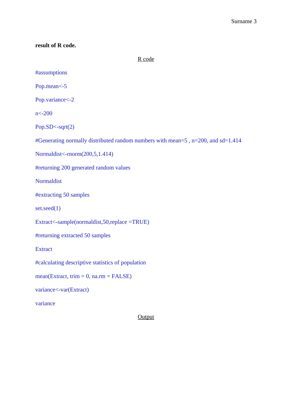
R code
#assumptions
Pop.mean<-5
Pop.variance<-2
n<-200
Pop.SD<-sqrt(2)
#Generating normally distributed random numbers with mean=5 , n=200, and sd=1.414
Normaldist<-rnorm(200,5,1.414)
#returning 200 generated random values
Normaldist
#extracting 50 samples
set.seed(1)
Extract<-sample(normaldist,50,replace =TRUE)
#returning extracted 50 samples
Extract
#calculating descriptive statistics of population
mean(Extract, trim = 0, na.rm = FALSE)
variance<-var(Extract)
variance
Output

Surname 4
The population (n=200) mean and variance is 5 and 2 respectively while the mean and
variance of the extracted sample is 5.03 and 1.62 respectively. The Sample mean and variance
are unbiased estimators of population mean and population variance respectively.1 The values
are very close to the actual population suggesting that mean and variance are unbiased
estimators of population mean and variance.
2. (Using R) If the X1 , ⋯ , X n N (μ , σ 2), and then consider a non-informative prior
distribution as the prior distribution of μ and σ 2. Let the prior distribution of μ and σ 2as
π ( μ , σ2 ) ∝ 1/σ2.
(a) Find the entire conditional posterior distribution of σ 2and β.
Assuming π ( μ , σ2 ) ∝ 1/σ2
Then conditional posterior distribution is calculated as:
π(μ , σ2|X) ∝ 1
σ−n−2 e
−1
2 σ 2 ∑
i=1
n
(X i−μ)2
1 Brani Vidakovic, Handout 5 (2018)

Surname 5
= 1
σ−n−2 e
−1
2 σ 2 [(n−1) s2+n (X −μ)2 ]
Where s2= 1
n−1 ∑
i=1
n
( X i−μ)2
Thus
The posterior distribution for α and β is given as:
θ|X~ IG(α + 1
2 , β + (μ−X )2
2 )
(b) (Using R) Use the Gibbs sampling method to extract samples from the posterior
distribution.
#declaring sample size
n = 20
#declaring nits= iterations
nits = 20000 #set number of iterations
#sample generated from N(1, 0.5)
x = rnorm(n, 1, sqrt(0.5))
xbar = mean(x)
s2 = var(x)
mu = c(1:nits)
psi = c(1:nits)
mu[1] = xbar #initiate chain using sample moments
psi[1] = 1/s2
for(i in 1:(nits-1)) {
+ psi[i+1] = rgamma(1, n/2, 0.5*sum((x-mu[i])*(x-mu[i])))
+ lam1 = ( n*psi[i+1])^-1*( psi[i+1]*sum(x))
+ lam2 = (n*psi[i+1])^-1

Surname 6
+ mu[i+1] = rnorm(1, lam1, sqrt(lam2))
+ }
#From my sequence of 20000 iterations we can get estimates of posterior means and
variances as:
mean(mu )
var(mu)
mean(psi)
var(psi)
#We estimate posterior probabilities P(mu > 1.5) and P(psi < 1.3333)
sum(mu > 1.5)/nits
#the probability is extremely small since the Markov chain never visits states for which mu >
1.5)
sum(psi<4/3)/nits
plot.ts(x)
acf(x)
(c) (Using R) Diagnose convergence using time-series plot and autocorrelation plot.

Surname 7
3. (Using R) If the X1 , ⋯ , X n N (μ , σ 2), and then consider semi-conjugate prior
distribution as the prior distribution of μ and σ 2. Let the prior distribution of μ as
N(0,100) and the prior distribution of σ−2 as Gamma(0 . 01 ,0 . 01).

Surname 8
(a) Find the entire conditional posterior distribution of σ 2and β.
Conditional conjugate prior distribution assumes that the random variables are independent
and identically distributed.2
If Xi| μ , σ2 ~ N( μ , σ2) are independent and identically distributed, and
Let σ 2 ~ IG( α,β)
Then
σ 2| x1, x2, x3,……, xn ~ IG(α + n
2 , β + 1
2 ∑ ¿ ¿)
Writing parametrically in terms of precisions, the semi-conjugate posterior is a gamma
distribution then,
P(τ ∨α , β) ∝ τ ( α + n
2 ) −1exp(−τ + 1
2 (β + 1
2 ∑(x1−μ) ))
(b) (Using R) Use the Gibbs sampling method to extract samples from the posterior
distribution.
#set sample size
n = 20
#set number of iterations
nits = 1000
#sample generated from N(0,100)
x = rnorm(n, 0, sqrt(100))
xbar = mean(x)
s2 = var(x)
mu = c(1:nits)
psi = c(1:nits)
2 Scott M Lynch, “Introduction to Applied Bayesian Statistics and Estimation for Social
Scientists (Springer, 2010).

Surname 9
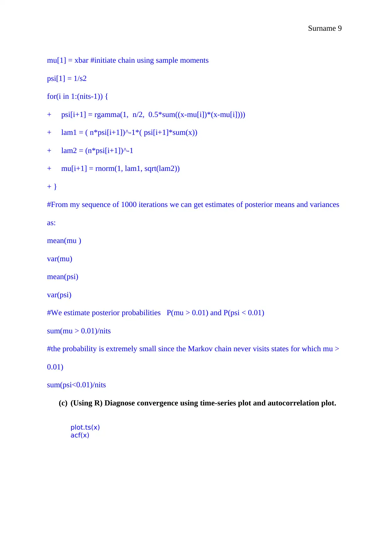
mu[1] = xbar #initiate chain using sample moments
psi[1] = 1/s2
for(i in 1:(nits-1)) {
+ psi[i+1] = rgamma(1, n/2, 0.5*sum((x-mu[i])*(x-mu[i])))
+ lam1 = ( n*psi[i+1])^-1*( psi[i+1]*sum(x))
+ lam2 = (n*psi[i+1])^-1
+ mu[i+1] = rnorm(1, lam1, sqrt(lam2))
+ }
#From my sequence of 1000 iterations we can get estimates of posterior means and variances
as:
mean(mu )
var(mu)
mean(psi)
var(psi)
#We estimate posterior probabilities P(mu > 0.01) and P(psi < 0.01)
sum(mu > 0.01)/nits
#the probability is extremely small since the Markov chain never visits states for which mu >
0.01)
sum(psi<0.01)/nits
(c) (Using R) Diagnose convergence using time-series plot and autocorrelation plot.
plot.ts(x)
acf(x)

Surname 10

Surname 11
Bibliography
Lynch, Scott M, Introduction to Applied Bayesian Statistics and Estimation for Social
Scientists (Springer, 2010)
Vidakovic, Brani, Handout 5 .Www2.isye.gatech.edu (2018)