Test for Difference in Mean Aggression, Thrill Seeking, and Risk Accepting
VerifiedAdded on 2023/01/19
|19
|3679
|60
AI Summary
This study examines the difference in mean aggression, thrill seeking, and risk accepting between different genders, metropolitan background statuses, and study modes.
Contribute Materials
Your contribution can guide someone’s learning journey. Share your
documents today.

Statistics
Statistics
Student name:
Tutor name:
1 | P a g e
Statistics
Student name:
Tutor name:
1 | P a g e
Secure Best Marks with AI Grader
Need help grading? Try our AI Grader for instant feedback on your assignments.
Statistics
NUMBER ONE
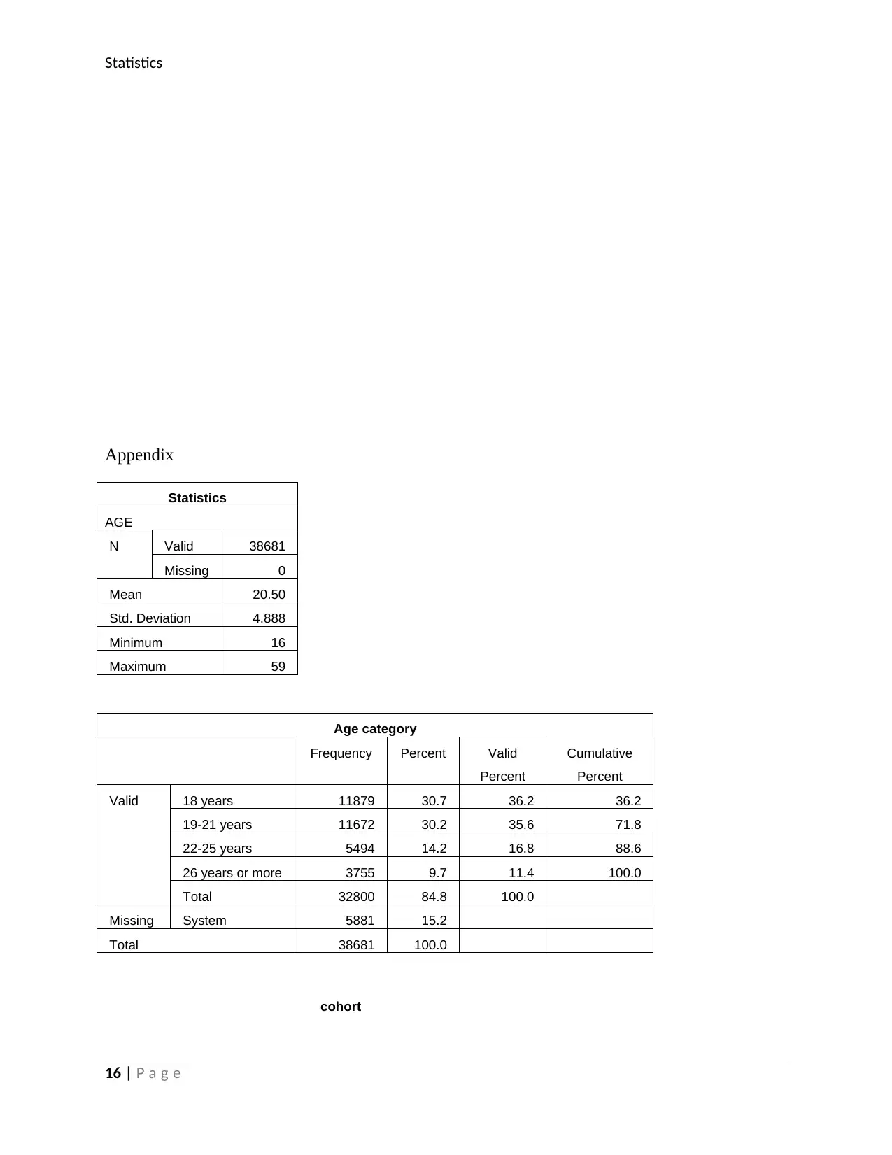
a. Descriptive statistics for age
Statistics
AGE
N Valid 38681
Missing 0
Mean 20.50
Std. Deviation 4.888
Minimum 16
Maximum 59
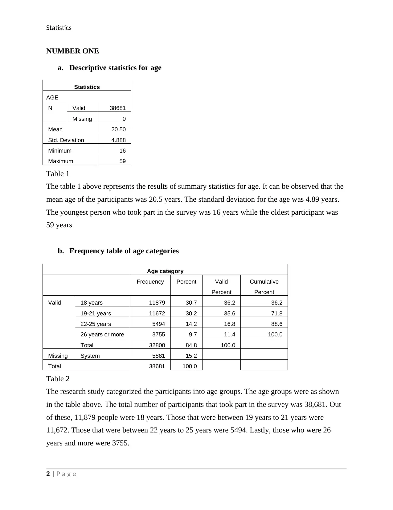
Table 1
The table 1 above represents the results of summary statistics for age. It can be observed that the
mean age of the participants was 20.5 years. The standard deviation for the age was 4.89 years.
The youngest person who took part in the survey was 16 years while the oldest participant was
59 years.
b. Frequency table of age categories
Age category
Frequency Percent Valid
Percent
Cumulative
Percent
Valid 18 years 11879 30.7 36.2 36.2
19-21 years 11672 30.2 35.6 71.8
22-25 years 5494 14.2 16.8 88.6
26 years or more 3755 9.7 11.4 100.0
Total 32800 84.8 100.0
Missing System 5881 15.2
Total 38681 100.0
Table 2
The research study categorized the participants into age groups. The age groups were as shown
in the table above. The total number of participants that took part in the survey was 38,681. Out
of these, 11,879 people were 18 years. Those that were between 19 years to 21 years were
11,672. Those that were between 22 years to 25 years were 5494. Lastly, those who were 26
years and more were 3755.
2 | P a g e
Statistics
QUESTION TWO
Tables of descriptive statistics
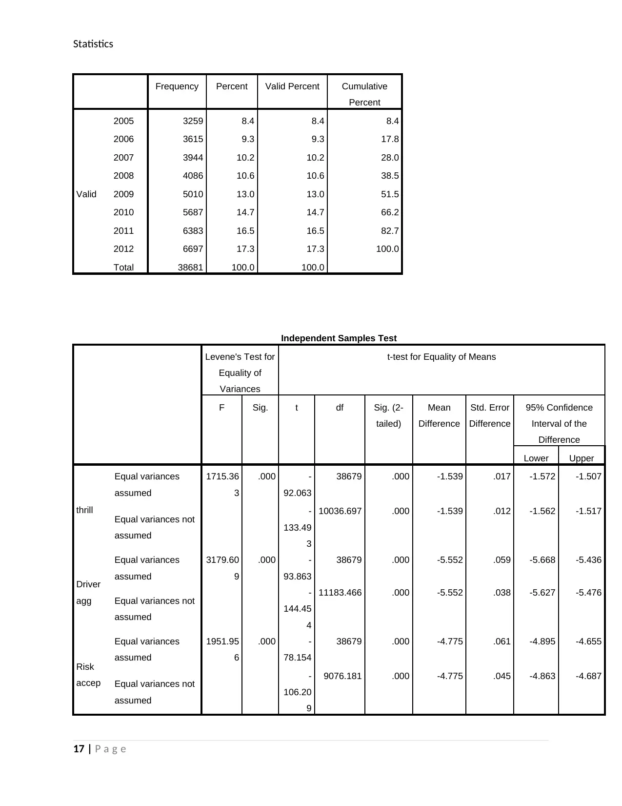
Cohort descriptive statistics table
cohort
Frequency Percent Valid Percent Cumulative
Percent
Valid
2005 3259 8.4 8.4 8.4
2006 3615 9.3 9.3 17.8
2007 3944 10.2 10.2 28.0
2008 4086 10.6 10.6 38.5
2009 5010 13.0 13.0 51.5
2010 5687 14.7 14.7 66.2
2011 6383 16.5 16.5 82.7
2012 6697 17.3 17.3 100.0
Total 38681 100.0 100.0
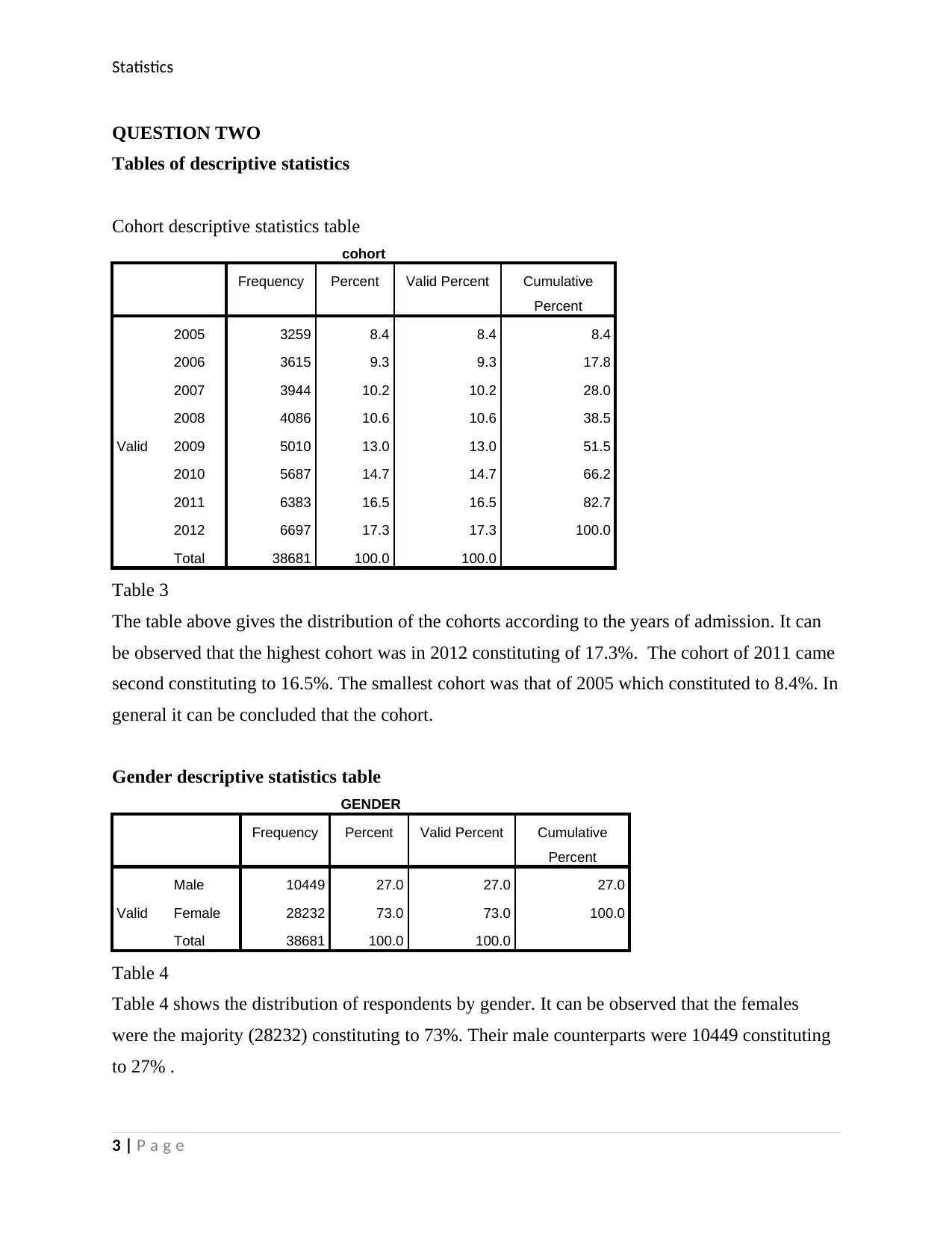
Table 3
The table above gives the distribution of the cohorts according to the years of admission. It can
be observed that the highest cohort was in 2012 constituting of 17.3%. The cohort of 2011 came
second constituting to 16.5%. The smallest cohort was that of 2005 which constituted to 8.4%. In
general it can be concluded that the cohort.
Gender descriptive statistics table
GENDER
Frequency Percent Valid Percent Cumulative
Percent
Valid
Male 10449 27.0 27.0 27.0
Female 28232 73.0 73.0 100.0
Total 38681 100.0 100.0
Table 4
Table 4 shows the distribution of respondents by gender. It can be observed that the females
were the majority (28232) constituting to 73%. Their male counterparts were 10449 constituting
to 27% .
3 | P a g e
Statistics
Living arrangement descriptive statistics table
LIVING_ARRANGE
Frequency Percent Valid Percent Cumulative
Percent
Valid
At home 20840 53.9 53.9 53.9
College/student accom 6850 17.7 17.7 71.6
Independently 10991 28.4 28.4 100.0
Total 38681 100.0 100.0
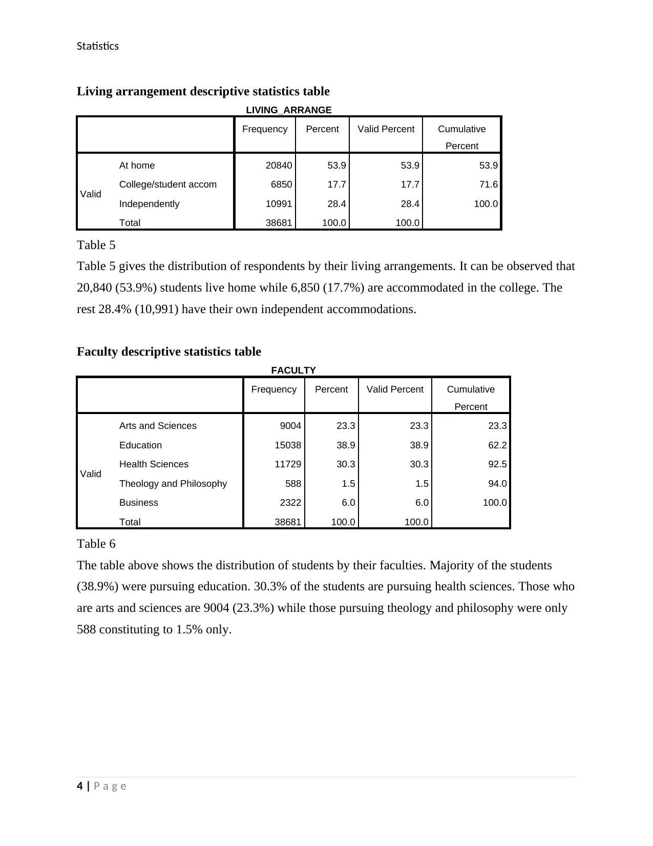
Table 5
Table 5 gives the distribution of respondents by their living arrangements. It can be observed that
20,840 (53.9%) students live home while 6,850 (17.7%) are accommodated in the college. The
rest 28.4% (10,991) have their own independent accommodations.
Faculty descriptive statistics table
FACULTY
Frequency Percent Valid Percent Cumulative
Percent
Valid
Arts and Sciences 9004 23.3 23.3 23.3
Education 15038 38.9 38.9 62.2
Health Sciences 11729 30.3 30.3 92.5
Theology and Philosophy 588 1.5 1.5 94.0
Business 2322 6.0 6.0 100.0
Total 38681 100.0 100.0
Table 6
The table above shows the distribution of students by their faculties. Majority of the students
(38.9%) were pursuing education. 30.3% of the students are pursuing health sciences. Those who
are arts and sciences are 9004 (23.3%) while those pursuing theology and philosophy were only
588 constituting to 1.5% only.
4 | P a g e
Secure Best Marks with AI Grader
Need help grading? Try our AI Grader for instant feedback on your assignments.
Statistics
Degree type descriptive statistics table
DEGREE_TYPE
Frequency Percent Valid Percent Cumulative
Percent
Valid
Single 34620 89.5 89.5 89.5
Double 4061 10.5 10.5 100.0
Total 38681 100.0 100.0
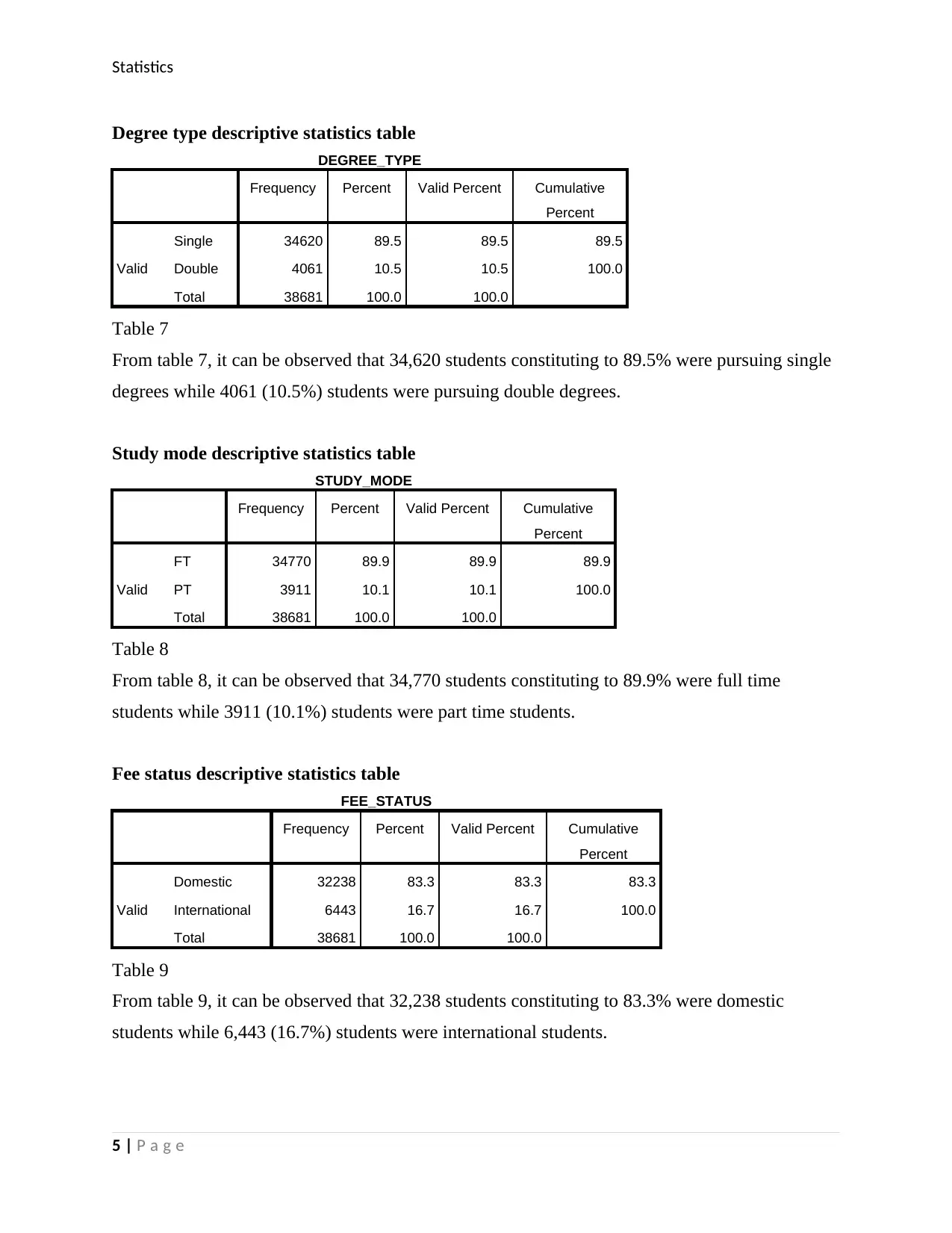
Table 7
From table 7, it can be observed that 34,620 students constituting to 89.5% were pursuing single
degrees while 4061 (10.5%) students were pursuing double degrees.
Study mode descriptive statistics table
STUDY_MODE
Frequency Percent Valid Percent Cumulative
Percent
Valid
FT 34770 89.9 89.9 89.9
PT 3911 10.1 10.1 100.0
Total 38681 100.0 100.0
Table 8
From table 8, it can be observed that 34,770 students constituting to 89.9% were full time
students while 3911 (10.1%) students were part time students.
Fee status descriptive statistics table
FEE_STATUS
Frequency Percent Valid Percent Cumulative
Percent
Valid
Domestic 32238 83.3 83.3 83.3
International 6443 16.7 16.7 100.0
Total 38681 100.0 100.0
Table 9
From table 9, it can be observed that 32,238 students constituting to 83.3% were domestic
students while 6,443 (16.7%) students were international students.
5 | P a g e
Statistics
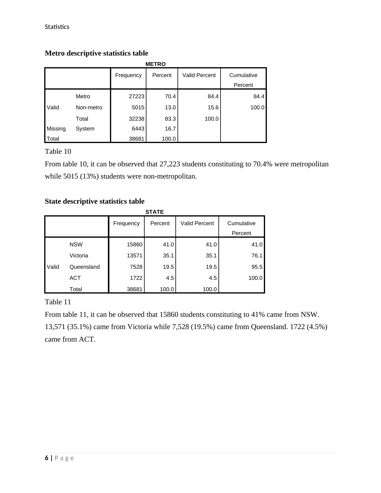
Metro descriptive statistics table
METRO
Frequency Percent Valid Percent Cumulative
Percent
Valid
Metro 27223 70.4 84.4 84.4
Non-metro 5015 13.0 15.6 100.0
Total 32238 83.3 100.0
Missing System 6443 16.7
Total 38681 100.0
Table 10
From table 10, it can be observed that 27,223 students constituting to 70.4% were metropolitan
while 5015 (13%) students were non-metropolitan.
State descriptive statistics table
STATE
Frequency Percent Valid Percent Cumulative
Percent
Valid
NSW 15860 41.0 41.0 41.0
Victoria 13571 35.1 35.1 76.1
Queensland 7528 19.5 19.5 95.5
ACT 1722 4.5 4.5 100.0
Total 38681 100.0 100.0
Table 11
From table 11, it can be observed that 15860 students constituting to 41% came from NSW.
13,571 (35.1%) came from Victoria while 7,528 (19.5%) came from Queensland. 1722 (4.5%)
came from ACT.
6 | P a g e
Statistics
NUMBER THREE
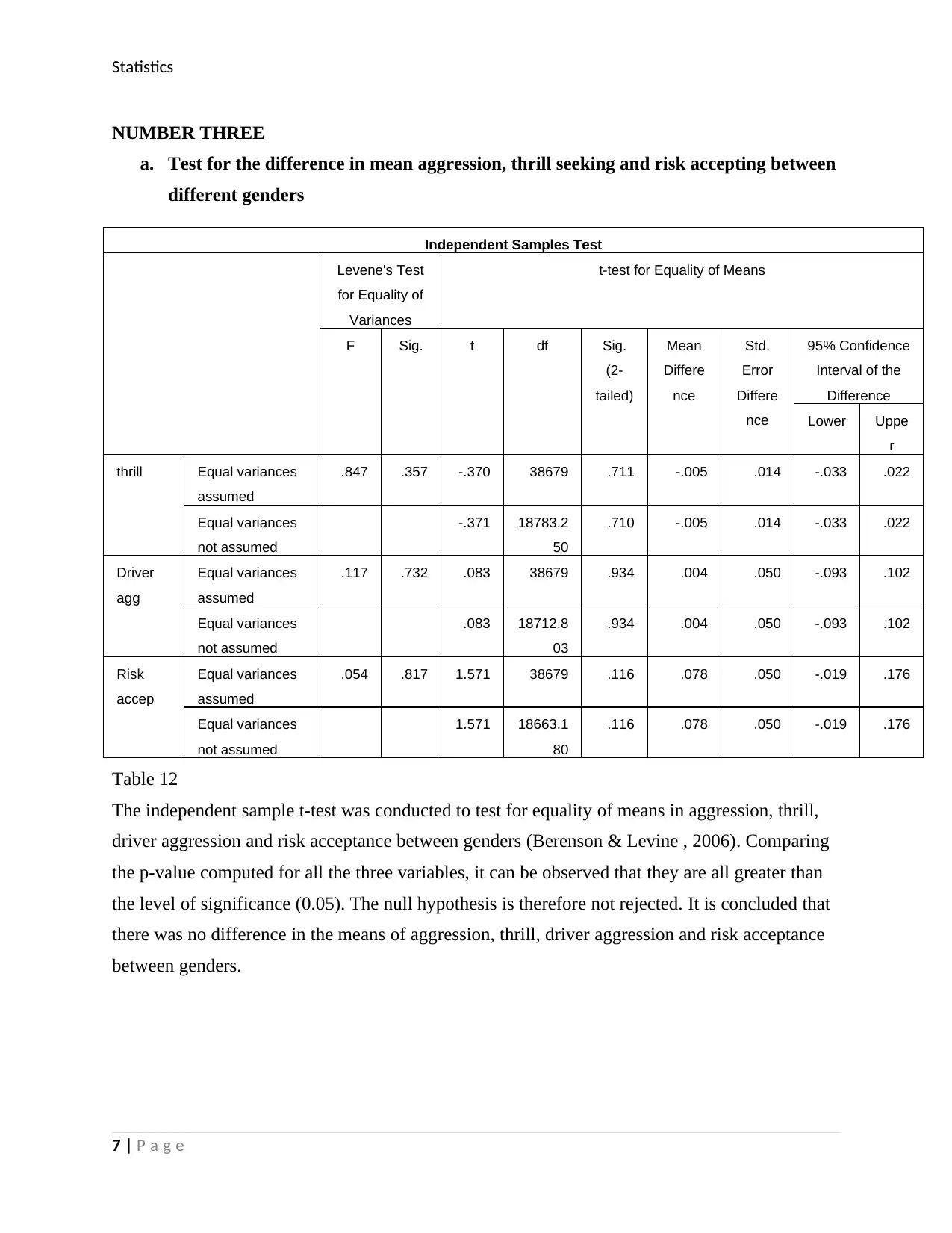
a. Test for the difference in mean aggression, thrill seeking and risk accepting between
different genders
Independent Samples Test
Levene's Test
for Equality of
Variances
t-test for Equality of Means
F Sig. t df Sig.
(2-
tailed)
Mean
Differe
nce
Std.
Error
Differe
nce
95% Confidence
Interval of the
Difference
Lower Uppe
r
thrill Equal variances
assumed
.847 .357 -.370 38679 .711 -.005 .014 -.033 .022
Equal variances
not assumed
-.371 18783.2
50
.710 -.005 .014 -.033 .022
Driver
agg
Equal variances
assumed
.117 .732 .083 38679 .934 .004 .050 -.093 .102
Equal variances
not assumed
.083 18712.8
03
.934 .004 .050 -.093 .102
Risk
accep
Equal variances
assumed
.054 .817 1.571 38679 .116 .078 .050 -.019 .176
Equal variances
not assumed
1.571 18663.1
80
.116 .078 .050 -.019 .176
Table 12
The independent sample t-test was conducted to test for equality of means in aggression, thrill,
driver aggression and risk acceptance between genders (Berenson & Levine , 2006). Comparing
the p-value computed for all the three variables, it can be observed that they are all greater than
the level of significance (0.05). The null hypothesis is therefore not rejected. It is concluded that
there was no difference in the means of aggression, thrill, driver aggression and risk acceptance
between genders.
7 | P a g e
Paraphrase This Document
Need a fresh take? Get an instant paraphrase of this document with our AI Paraphraser
Statistics
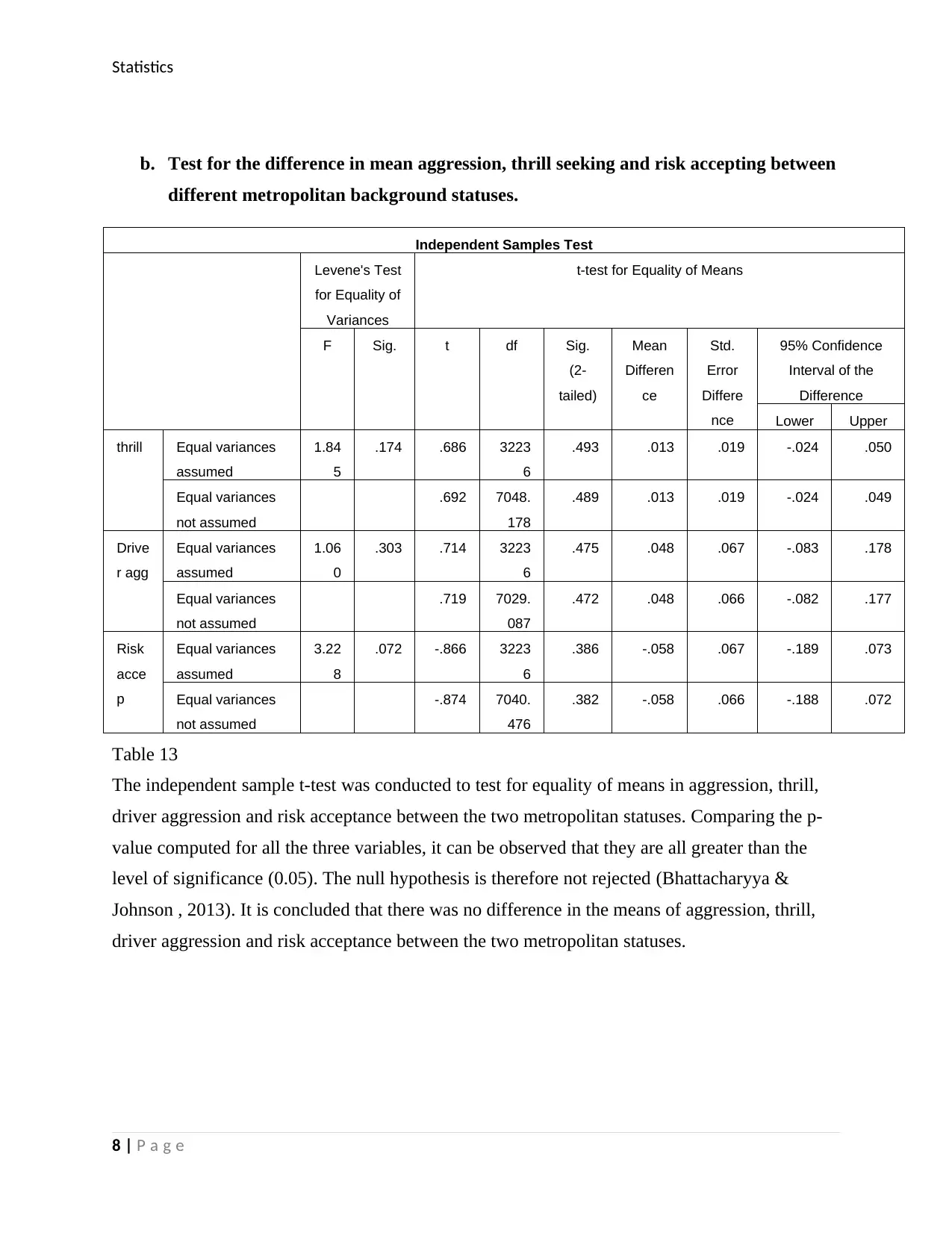
b. Test for the difference in mean aggression, thrill seeking and risk accepting between
different metropolitan background statuses.
Independent Samples Test
Levene's Test
for Equality of
Variances
t-test for Equality of Means
F Sig. t df Sig.
(2-
tailed)
Mean
Differen
ce
Std.
Error
Differe
nce
95% Confidence
Interval of the
Difference
Lower Upper
thrill Equal variances
assumed
1.84
5
.174 .686 3223
6
.493 .013 .019 -.024 .050
Equal variances
not assumed
.692 7048.
178
.489 .013 .019 -.024 .049
Drive
r agg
Equal variances
assumed
1.06
0
.303 .714 3223
6
.475 .048 .067 -.083 .178
Equal variances
not assumed
.719 7029.
087
.472 .048 .066 -.082 .177
Risk
acce
p
Equal variances
assumed
3.22
8
.072 -.866 3223
6
.386 -.058 .067 -.189 .073
Equal variances
not assumed
-.874 7040.
476
.382 -.058 .066 -.188 .072
Table 13
The independent sample t-test was conducted to test for equality of means in aggression, thrill,
driver aggression and risk acceptance between the two metropolitan statuses. Comparing the p-
value computed for all the three variables, it can be observed that they are all greater than the
level of significance (0.05). The null hypothesis is therefore not rejected (Bhattacharyya &
Johnson , 2013). It is concluded that there was no difference in the means of aggression, thrill,
driver aggression and risk acceptance between the two metropolitan statuses.
8 | P a g e
Statistics
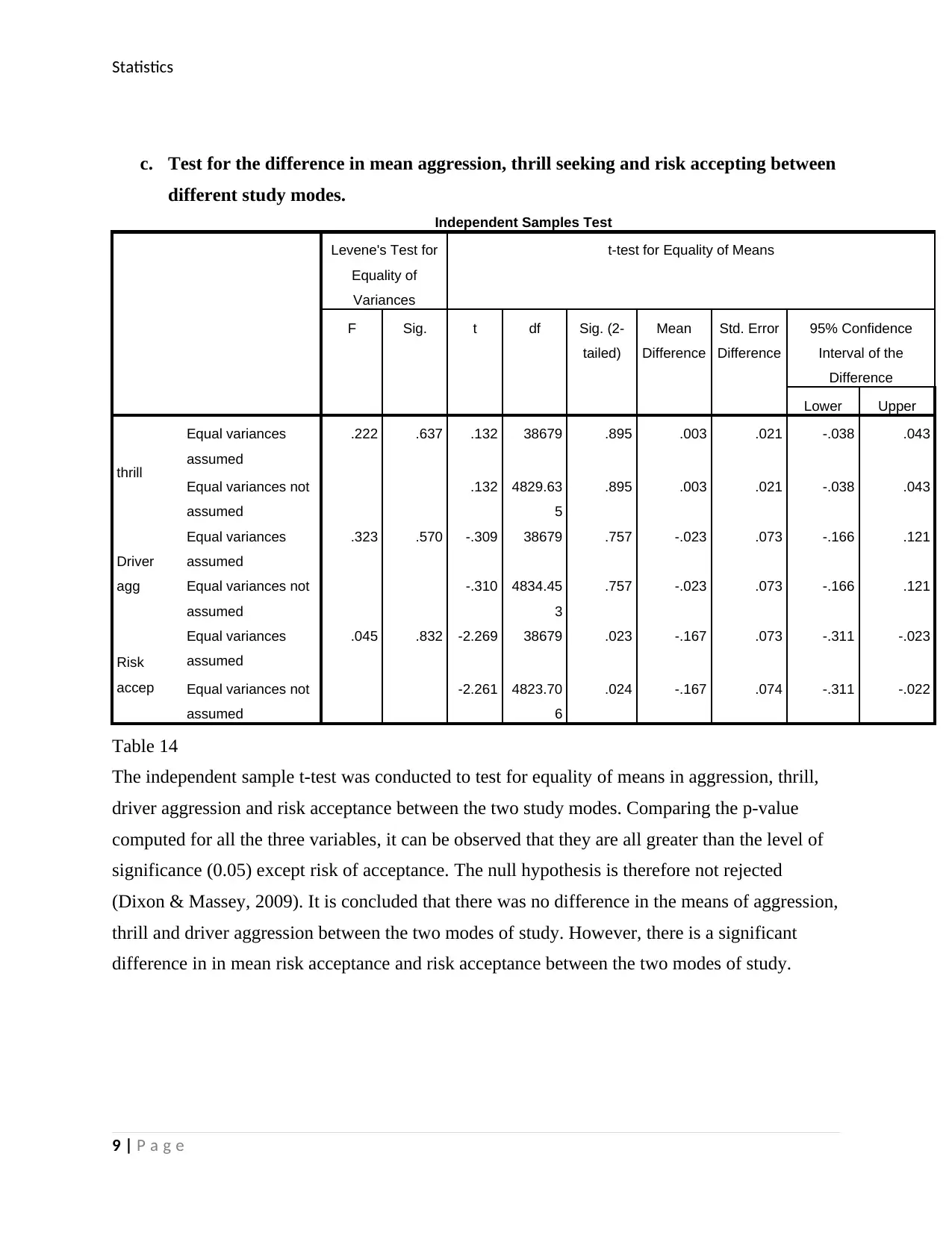
c. Test for the difference in mean aggression, thrill seeking and risk accepting between
different study modes.
Independent Samples Test
Levene's Test for
Equality of
Variances
t-test for Equality of Means
F Sig. t df Sig. (2-
tailed)
Mean
Difference
Std. Error
Difference
95% Confidence
Interval of the
Difference
Lower Upper
thrill
Equal variances
assumed
.222 .637 .132 38679 .895 .003 .021 -.038 .043
Equal variances not
assumed
.132 4829.63
5
.895 .003 .021 -.038 .043
Driver
agg
Equal variances
assumed
.323 .570 -.309 38679 .757 -.023 .073 -.166 .121
Equal variances not
assumed
-.310 4834.45
3
.757 -.023 .073 -.166 .121
Risk
accep
Equal variances
assumed
.045 .832 -2.269 38679 .023 -.167 .073 -.311 -.023
Equal variances not
assumed
-2.261 4823.70
6
.024 -.167 .074 -.311 -.022
Table 14
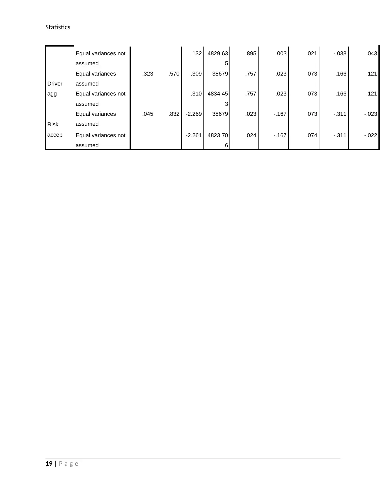
The independent sample t-test was conducted to test for equality of means in aggression, thrill,
driver aggression and risk acceptance between the two study modes. Comparing the p-value
computed for all the three variables, it can be observed that they are all greater than the level of
significance (0.05) except risk of acceptance. The null hypothesis is therefore not rejected
(Dixon & Massey, 2009). It is concluded that there was no difference in the means of aggression,
thrill and driver aggression between the two modes of study. However, there is a significant
difference in in mean risk acceptance and risk acceptance between the two modes of study.
9 | P a g e
Statistics
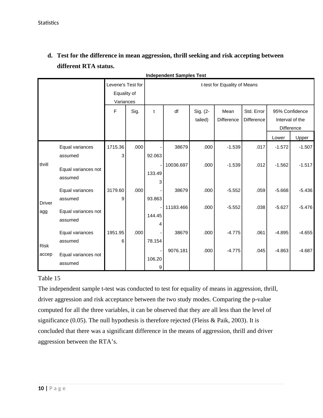
d. Test for the difference in mean aggression, thrill seeking and risk accepting between
different RTA status.
Independent Samples Test
Levene's Test for
Equality of
Variances
t-test for Equality of Means
F Sig. t df Sig. (2-
tailed)
Mean
Difference
Std. Error
Difference
95% Confidence
Interval of the
Difference
Lower Upper
thrill
Equal variances
assumed
1715.36
3
.000 -
92.063
38679 .000 -1.539 .017 -1.572 -1.507
Equal variances not
assumed
-
133.49
3
10036.697 .000 -1.539 .012 -1.562 -1.517
Driver
agg
Equal variances
assumed
3179.60
9
.000 -
93.863
38679 .000 -5.552 .059 -5.668 -5.436
Equal variances not
assumed
-
144.45
4
11183.466 .000 -5.552 .038 -5.627 -5.476
Risk
accep
Equal variances
assumed
1951.95
6
.000 -
78.154
38679 .000 -4.775 .061 -4.895 -4.655
Equal variances not
assumed
-
106.20
9
9076.181 .000 -4.775 .045 -4.863 -4.687
Table 15
The independent sample t-test was conducted to test for equality of means in aggression, thrill,
driver aggression and risk acceptance between the two study modes. Comparing the p-value
computed for all the three variables, it can be observed that they are all less than the level of
significance (0.05). The null hypothesis is therefore rejected (Fleiss & Paik, 2003). It is
concluded that there was a significant difference in the means of aggression, thrill and driver
aggression between the RTA’s.
10 | P a g e
Secure Best Marks with AI Grader
Need help grading? Try our AI Grader for instant feedback on your assignments.
Statistics
QUESTION FOUR
a. Test for the difference in depression status by gender
Independent Samples Test
Levene's Test for
Equality of
Variances
t-test for Equality of Means
F Sig. t df Sig. (2-
tailed)
Mean
Difference
Std. Error
Difference
95% Confidence
Interval of the
Difference
Lower Upper
GENDER
Equal variances
assumed
1.104 .293 .529 38679 .597 .00394 .00745 -.01066 .01854
Equal variances
not assumed
.527 4898.622 .598 .00394 .00747 -.01071 .01859
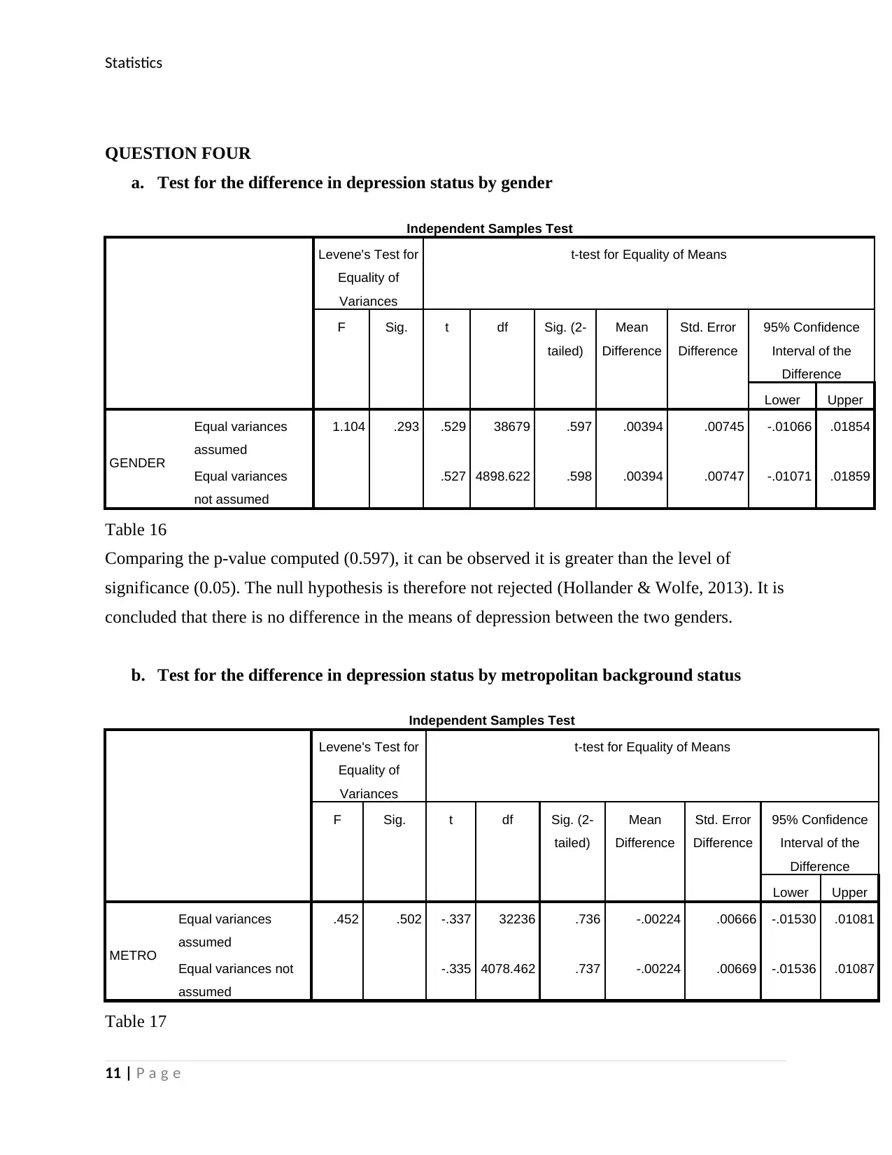
Table 16
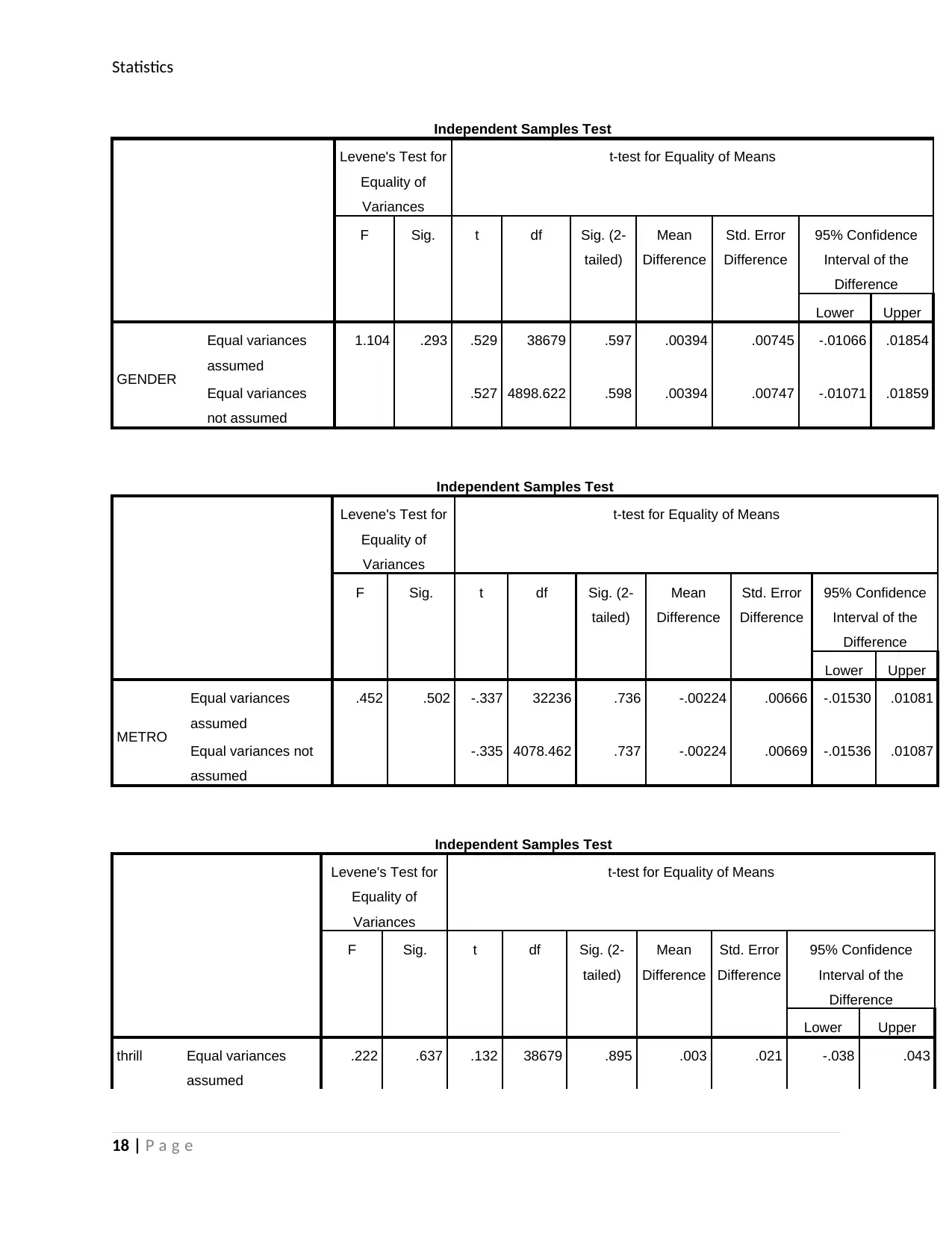
Comparing the p-value computed (0.597), it can be observed it is greater than the level of
significance (0.05). The null hypothesis is therefore not rejected (Hollander & Wolfe, 2013). It is
concluded that there is no difference in the means of depression between the two genders.
b. Test for the difference in depression status by metropolitan background status
Independent Samples Test
Levene's Test for
Equality of
Variances
t-test for Equality of Means
F Sig. t df Sig. (2-
tailed)
Mean
Difference
Std. Error
Difference
95% Confidence
Interval of the
Difference
Lower Upper
METRO
Equal variances
assumed
.452 .502 -.337 32236 .736 -.00224 .00666 -.01530 .01081
Equal variances not
assumed
-.335 4078.462 .737 -.00224 .00669 -.01536 .01087
Table 17
11 | P a g e
Statistics
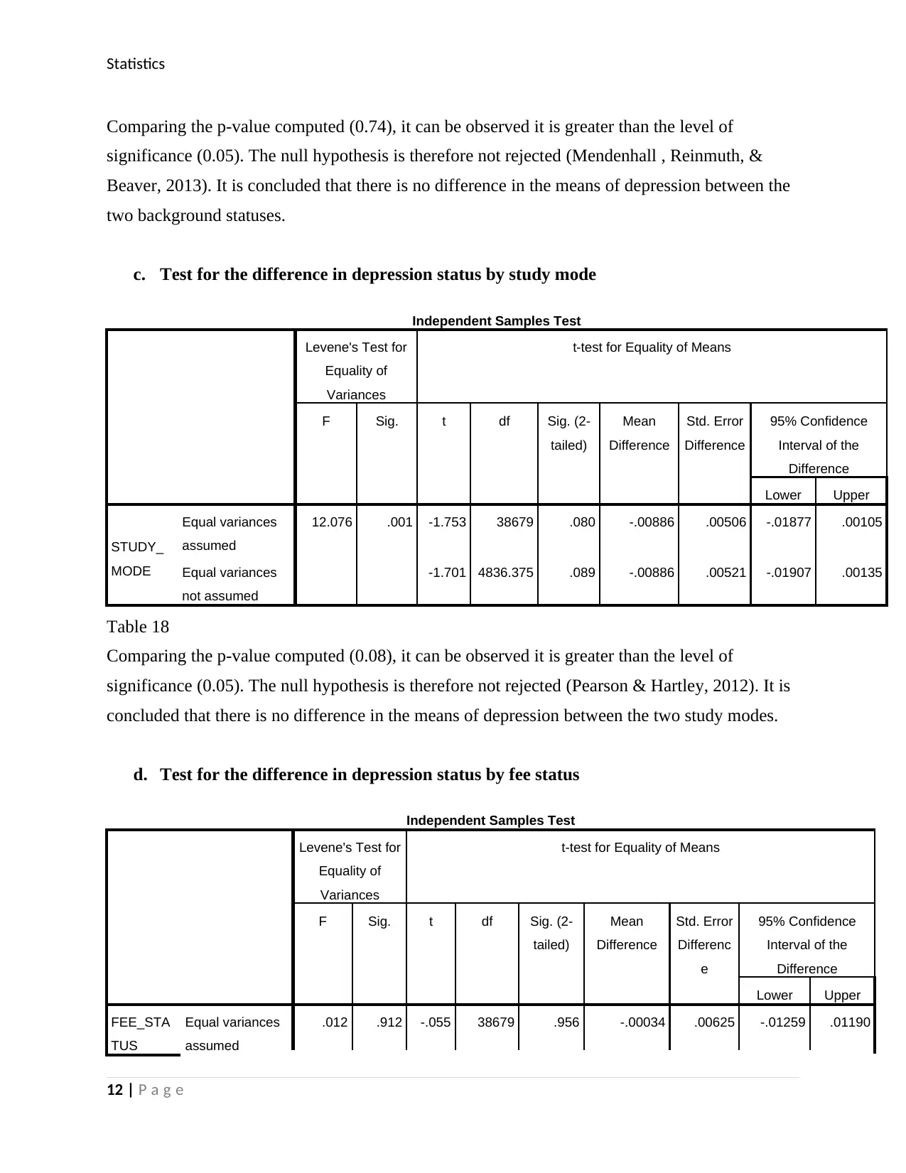
Comparing the p-value computed (0.74), it can be observed it is greater than the level of
significance (0.05). The null hypothesis is therefore not rejected (Mendenhall , Reinmuth, &
Beaver, 2013). It is concluded that there is no difference in the means of depression between the
two background statuses.
c. Test for the difference in depression status by study mode
Independent Samples Test
Levene's Test for
Equality of
Variances
t-test for Equality of Means
F Sig. t df Sig. (2-
tailed)
Mean
Difference
Std. Error
Difference
95% Confidence
Interval of the
Difference
Lower Upper
STUDY_
MODE
Equal variances
assumed
12.076 .001 -1.753 38679 .080 -.00886 .00506 -.01877 .00105
Equal variances
not assumed
-1.701 4836.375 .089 -.00886 .00521 -.01907 .00135
Table 18
Comparing the p-value computed (0.08), it can be observed it is greater than the level of
significance (0.05). The null hypothesis is therefore not rejected (Pearson & Hartley, 2012). It is
concluded that there is no difference in the means of depression between the two study modes.
d. Test for the difference in depression status by fee status
Independent Samples Test
Levene's Test for
Equality of
Variances
t-test for Equality of Means
F Sig. t df Sig. (2-
tailed)
Mean
Difference
Std. Error
Differenc
e
95% Confidence
Interval of the
Difference
Lower Upper
FEE_STA
TUS
Equal variances
assumed
.012 .912 -.055 38679 .956 -.00034 .00625 -.01259 .01190
12 | P a g e
Statistics
Equal variances
not assumed
-.055 4905.94
2
.956 -.00034 .00625 -.01260 .01191
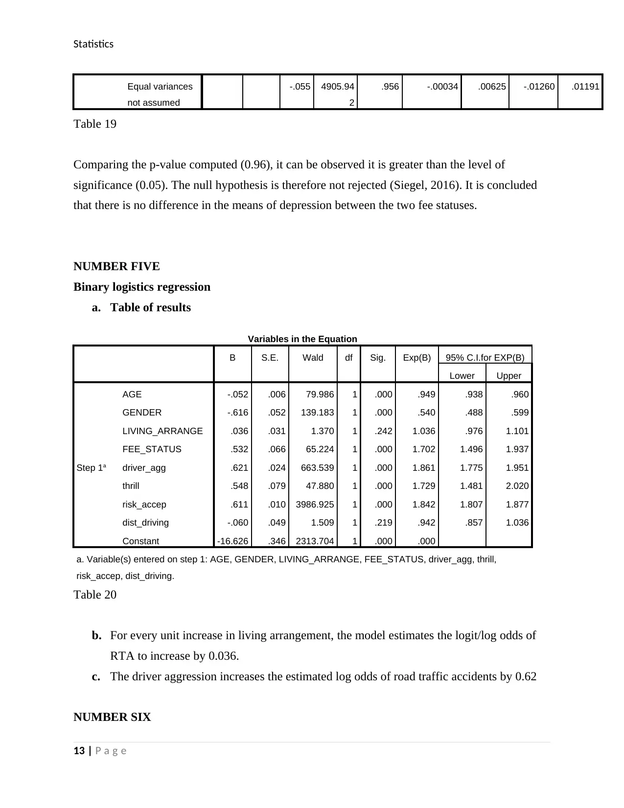
Table 19
Comparing the p-value computed (0.96), it can be observed it is greater than the level of
significance (0.05). The null hypothesis is therefore not rejected (Siegel, 2016). It is concluded
that there is no difference in the means of depression between the two fee statuses.
NUMBER FIVE
Binary logistics regression
a. Table of results
Variables in the Equation
B S.E. Wald df Sig. Exp(B) 95% C.I.for EXP(B)
Lower Upper
Step 1a
AGE -.052 .006 79.986 1 .000 .949 .938 .960
GENDER -.616 .052 139.183 1 .000 .540 .488 .599
LIVING_ARRANGE .036 .031 1.370 1 .242 1.036 .976 1.101
FEE_STATUS .532 .066 65.224 1 .000 1.702 1.496 1.937
driver_agg .621 .024 663.539 1 .000 1.861 1.775 1.951
thrill .548 .079 47.880 1 .000 1.729 1.481 2.020
risk_accep .611 .010 3986.925 1 .000 1.842 1.807 1.877
dist_driving -.060 .049 1.509 1 .219 .942 .857 1.036
Constant -16.626 .346 2313.704 1 .000 .000
a. Variable(s) entered on step 1: AGE, GENDER, LIVING_ARRANGE, FEE_STATUS, driver_agg, thrill,
risk_accep, dist_driving.
Table 20
b. For every unit increase in living arrangement, the model estimates the logit/log odds of
RTA to increase by 0.036.
c. The driver aggression increases the estimated log odds of road traffic accidents by 0.62
NUMBER SIX
13 | P a g e
Paraphrase This Document
Need a fresh take? Get an instant paraphrase of this document with our AI Paraphraser
Statistics
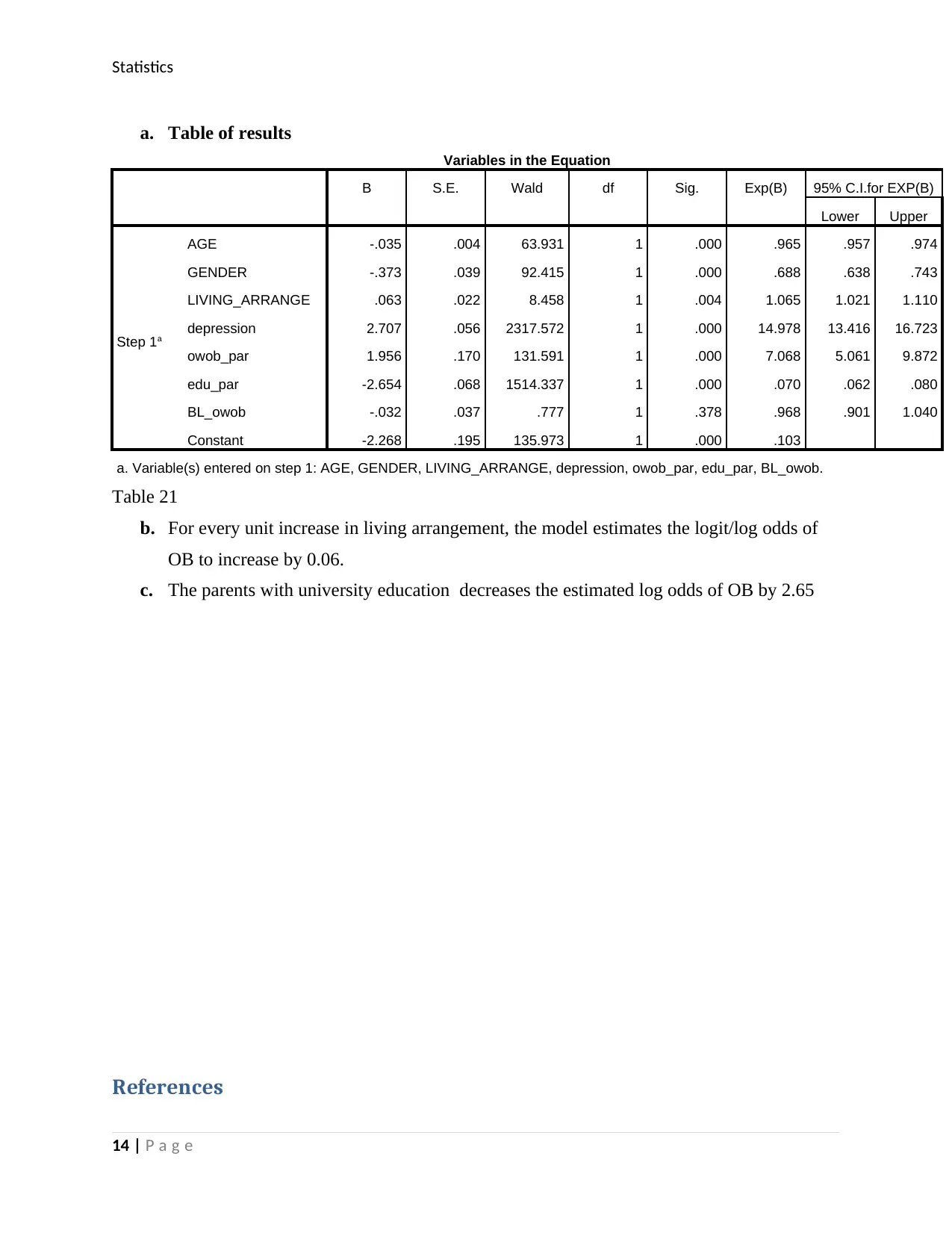
a. Table of results
Variables in the Equation
B S.E. Wald df Sig. Exp(B) 95% C.I.for EXP(B)
Lower Upper
Step 1a
AGE -.035 .004 63.931 1 .000 .965 .957 .974
GENDER -.373 .039 92.415 1 .000 .688 .638 .743
LIVING_ARRANGE .063 .022 8.458 1 .004 1.065 1.021 1.110
depression 2.707 .056 2317.572 1 .000 14.978 13.416 16.723
owob_par 1.956 .170 131.591 1 .000 7.068 5.061 9.872
edu_par -2.654 .068 1514.337 1 .000 .070 .062 .080
BL_owob -.032 .037 .777 1 .378 .968 .901 1.040
Constant -2.268 .195 135.973 1 .000 .103
a. Variable(s) entered on step 1: AGE, GENDER, LIVING_ARRANGE, depression, owob_par, edu_par, BL_owob.
Table 21
b. For every unit increase in living arrangement, the model estimates the logit/log odds of
OB to increase by 0.06.
c. The parents with university education decreases the estimated log odds of OB by 2.65
References
14 | P a g e
Statistics
Statistics for Management and Economics, Duxbury Press, Belmont, CA. (n.d.).
Berenson, M. L., & Levine , D. M. (2006). Basic Business Statistics. New Jersey: Prentice-Hall, Englewood
Cliffs.
Bhattacharyya, G. K., & Johnson , R. A. (2013). Statistical Concepts and Methods. New York: John Wiley
and Sons.
Dixon , W. J., & Massey, F. J. (2009). Introduction to Statistical Analysis. New York: McGraw-Hill.
Fleiss, J. L., & Paik, M. C. (2003). Statistical Methods for Rates and Proportions, Third Edition,. New York:
John Wiley & Sons.
Hicks, C. R. (2013). Fundamental Concepts in the Design of Experiments. New-York: Rhinehart and
Winston.
Hollander , M., & Wolfe, D. A. (2013). Nonparametric Statistical Methods. New York: John Wiley & Sons.
Mendenhall , W., Reinmuth, J. E., & Beaver, R. J. (2013). Statistics for Management and Economics.
Belmont, CA: Duxbury Press.
Neter , J. N., & Whitmore , R. M. (2014). Applied Statistics. Boston, MA.: Allyn and Bacon.
Pearson, A. V., & Hartley, H. O. (2012). Biometrica Tables for Statisticians. Cambridge: Cambridge
University Press.
Siegel, S. (2016). Nonparametric Statistics. New York: McGraw-Hill.
15 | P a g e
Statistics
Appendix
Statistics
AGE
N Valid 38681
Missing 0
Mean 20.50
Std. Deviation 4.888
Minimum 16
Maximum 59
Age category
Frequency Percent Valid
Percent
Cumulative
Percent
Valid 18 years 11879 30.7 36.2 36.2
19-21 years 11672 30.2 35.6 71.8
22-25 years 5494 14.2 16.8 88.6
26 years or more 3755 9.7 11.4 100.0
Total 32800 84.8 100.0
Missing System 5881 15.2
Total 38681 100.0
cohort
16 | P a g e
Secure Best Marks with AI Grader
Need help grading? Try our AI Grader for instant feedback on your assignments.
Statistics
Frequency Percent Valid Percent Cumulative
Percent
Valid
2005 3259 8.4 8.4 8.4
2006 3615 9.3 9.3 17.8
2007 3944 10.2 10.2 28.0
2008 4086 10.6 10.6 38.5
2009 5010 13.0 13.0 51.5
2010 5687 14.7 14.7 66.2
2011 6383 16.5 16.5 82.7
2012 6697 17.3 17.3 100.0
Total 38681 100.0 100.0
Independent Samples Test
Levene's Test for
Equality of
Variances
t-test for Equality of Means
F Sig. t df Sig. (2-
tailed)
Mean
Difference
Std. Error
Difference
95% Confidence
Interval of the
Difference
Lower Upper
thrill
Equal variances
assumed
1715.36
3
.000 -
92.063
38679 .000 -1.539 .017 -1.572 -1.507
Equal variances not
assumed
-
133.49
3
10036.697 .000 -1.539 .012 -1.562 -1.517
Driver
agg
Equal variances
assumed
3179.60
9
.000 -
93.863
38679 .000 -5.552 .059 -5.668 -5.436
Equal variances not
assumed
-
144.45
4
11183.466 .000 -5.552 .038 -5.627 -5.476
Risk
accep
Equal variances
assumed
1951.95
6
.000 -
78.154
38679 .000 -4.775 .061 -4.895 -4.655
Equal variances not
assumed
-
106.20
9
9076.181 .000 -4.775 .045 -4.863 -4.687
17 | P a g e
Statistics
Independent Samples Test
Levene's Test for
Equality of
Variances
t-test for Equality of Means
F Sig. t df Sig. (2-
tailed)
Mean
Difference
Std. Error
Difference
95% Confidence
Interval of the
Difference
Lower Upper
GENDER
Equal variances
assumed
1.104 .293 .529 38679 .597 .00394 .00745 -.01066 .01854
Equal variances
not assumed
.527 4898.622 .598 .00394 .00747 -.01071 .01859
Independent Samples Test
Levene's Test for
Equality of
Variances
t-test for Equality of Means
F Sig. t df Sig. (2-
tailed)
Mean
Difference
Std. Error
Difference
95% Confidence
Interval of the
Difference
Lower Upper
METRO
Equal variances
assumed
.452 .502 -.337 32236 .736 -.00224 .00666 -.01530 .01081
Equal variances not
assumed
-.335 4078.462 .737 -.00224 .00669 -.01536 .01087
Independent Samples Test
Levene's Test for
Equality of
Variances
t-test for Equality of Means
F Sig. t df Sig. (2-
tailed)
Mean
Difference
Std. Error
Difference
95% Confidence
Interval of the
Difference
Lower Upper
thrill Equal variances
assumed
.222 .637 .132 38679 .895 .003 .021 -.038 .043
18 | P a g e
Independent Samples Test
Levene's Test for
Equality of
Variances
t-test for Equality of Means
F Sig. t df Sig. (2-
tailed)
Mean
Difference
Std. Error
Difference
95% Confidence
Interval of the
Difference
Lower Upper
GENDER
Equal variances
assumed
1.104 .293 .529 38679 .597 .00394 .00745 -.01066 .01854
Equal variances
not assumed
.527 4898.622 .598 .00394 .00747 -.01071 .01859
Independent Samples Test
Levene's Test for
Equality of
Variances
t-test for Equality of Means
F Sig. t df Sig. (2-
tailed)
Mean
Difference
Std. Error
Difference
95% Confidence
Interval of the
Difference
Lower Upper
METRO
Equal variances
assumed
.452 .502 -.337 32236 .736 -.00224 .00666 -.01530 .01081
Equal variances not
assumed
-.335 4078.462 .737 -.00224 .00669 -.01536 .01087
Independent Samples Test
Levene's Test for
Equality of
Variances
t-test for Equality of Means
F Sig. t df Sig. (2-
tailed)
Mean
Difference
Std. Error
Difference
95% Confidence
Interval of the
Difference
Lower Upper
thrill Equal variances
assumed
.222 .637 .132 38679 .895 .003 .021 -.038 .043
18 | P a g e
Statistics
Equal variances not
assumed
.132 4829.63
5
.895 .003 .021 -.038 .043
Driver
agg
Equal variances
assumed
.323 .570 -.309 38679 .757 -.023 .073 -.166 .121
Equal variances not
assumed
-.310 4834.45
3
.757 -.023 .073 -.166 .121
Risk
accep
Equal variances
assumed
.045 .832 -2.269 38679 .023 -.167 .073 -.311 -.023
Equal variances not
assumed
-2.261 4823.70
6
.024 -.167 .074 -.311 -.022
19 | P a g e
Equal variances not
assumed
.132 4829.63
5
.895 .003 .021 -.038 .043
Driver
agg
Equal variances
assumed
.323 .570 -.309 38679 .757 -.023 .073 -.166 .121
Equal variances not
assumed
-.310 4834.45
3
.757 -.023 .073 -.166 .121
Risk
accep
Equal variances
assumed
.045 .832 -2.269 38679 .023 -.167 .073 -.311 -.023
Equal variances not
assumed
-2.261 4823.70
6
.024 -.167 .074 -.311 -.022
19 | P a g e
1 out of 19
Related Documents
Your All-in-One AI-Powered Toolkit for Academic Success.
+13062052269
info@desklib.com
Available 24*7 on WhatsApp / Email
![[object Object]](/_next/static/media/star-bottom.7253800d.svg)
Unlock your academic potential
© 2024 | Zucol Services PVT LTD | All rights reserved.


