Student Weight Gain Analysis

This assignment delves into the relationship between student weight across two semesters. It presents descriptive statistics comparing male and female student weights, analyzes correlations between semester-to-semester weight changes, and employs Chi-Square tests to determine statistically significant associations. The research concludes with recommendations for improved data reporting and analysis regarding student weight fluctuations.

1
Title
Student Name
Course
Professor Name
Date Submitted

2
Introduction
Weight gain and obesity has become a key issue for people throughout the world.
This weight gain among young university or college students has become a vital concern.
Furthermore, there is also increased anxiety about if weight of male and female differ from
each other. It is believed that weight of female is slightly higher than male from age group of
7 to 16 but weight of male are slightly higher than weight of male after age 18, i.e. when they
reach in college or university level (Halls, 2017). Furthermore in late adolescents’ years,
transition from high secondary to university is critical and vulnerable period for changes in
body weight and unhealthy lifestyle adoption (Vadeboncoeur, 2015). Based on this aspect,
the research is going to analyse if there is difference between average weight of male and
female students. Furthermore, the research is also going to analyse if there is difference in
weight of students in first and second semester.
Research Design
The research is based on descriptive design. The key objective of the research is to
determine the frequency of occurrence, which is in this case the weight of students. It
evaluates the covariance between the variables. It is basically a longitudinal study, which
involves drawing samples from population that are assessed repeatedly through time
(Sreejesh, 2013).
There are two research questions which have been analysed in the study which are:
1. Is the average weight of male students significantly higher than the average weight of
female students? and
2. Is the weight of student the same during the first semester and during the second
semester?

3
Based on the research questions, the following hypotheses are tested:
The first hypothesis of the research is:
H1: There is relationship between the weight of female and male students
H0: There is no relationship between the weight of female and male students
The second hypothesis of the research is:
H2: There is relationship between the weight of students in first semester and second
semester
H0: There is no relationship between the weight of students in first semester and
second semester
In order to analyse the hypothesis, about 100 respondents from each sample has been
observed. The hypothesis has been evaluated by using statistical measures. Bivariate tests
comprising independent sample t test, paired samples t test, one way Anova, correlation and
chi square test has been used in order to assess the hypothesis. Popular application MS Excel
has been used in order to analyse the research questions and hypotheses.

4
Results and Discussion
Analysis of First Question/Hypothesis
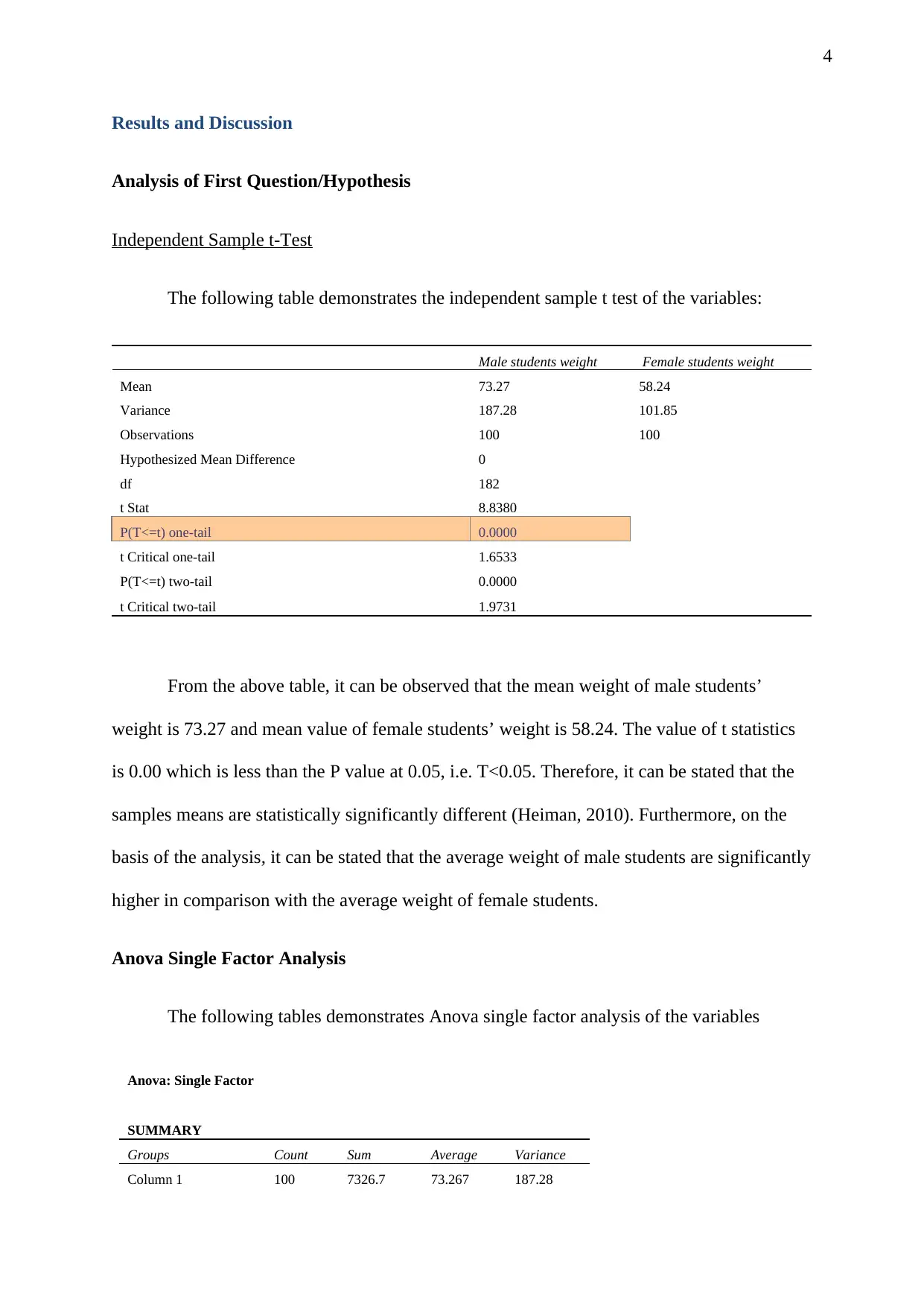
Independent Sample t-Test
The following table demonstrates the independent sample t test of the variables:
Male students weight Female students weight
Mean 73.27 58.24
Variance 187.28 101.85
Observations 100 100
Hypothesized Mean Difference 0
df 182
t Stat 8.8380
P(T<=t) one-tail 0.0000
t Critical one-tail 1.6533
P(T<=t) two-tail 0.0000
t Critical two-tail 1.9731
From the above table, it can be observed that the mean weight of male students’
weight is 73.27 and mean value of female students’ weight is 58.24. The value of t statistics
is 0.00 which is less than the P value at 0.05, i.e. T<0.05. Therefore, it can be stated that the
samples means are statistically significantly different (Heiman, 2010). Furthermore, on the
basis of the analysis, it can be stated that the average weight of male students are significantly
higher in comparison with the average weight of female students.
Anova Single Factor Analysis
The following tables demonstrates Anova single factor analysis of the variables
Anova: Single Factor
SUMMARY
Groups Count Sum Average Variance
Column 1 100 7326.7 73.267 187.28

5
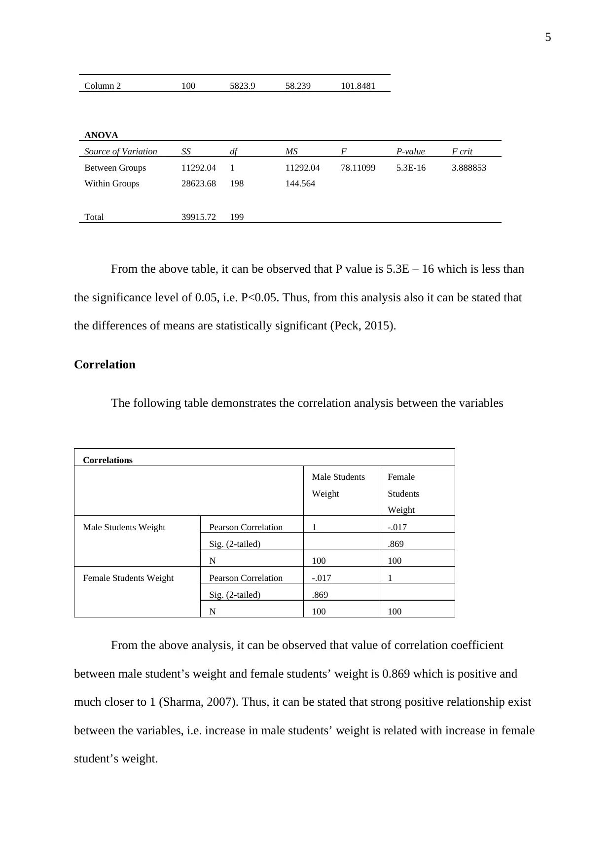
Column 2 100 5823.9 58.239 101.8481
ANOVA
Source of Variation SS df MS F P-value F crit
Between Groups 11292.04 1 11292.04 78.11099 5.3E-16 3.888853
Within Groups 28623.68 198 144.564
Total 39915.72 199
From the above table, it can be observed that P value is 5.3E – 16 which is less than
the significance level of 0.05, i.e. P<0.05. Thus, from this analysis also it can be stated that
the differences of means are statistically significant (Peck, 2015).
Correlation
The following table demonstrates the correlation analysis between the variables
Correlations
Male Students
Weight
Female
Students
Weight
Male Students Weight Pearson Correlation 1 -.017
Sig. (2-tailed) .869
N 100 100
Female Students Weight Pearson Correlation -.017 1
Sig. (2-tailed) .869
N 100 100
From the above analysis, it can be observed that value of correlation coefficient
between male student’s weight and female students’ weight is 0.869 which is positive and
much closer to 1 (Sharma, 2007). Thus, it can be stated that strong positive relationship exist
between the variables, i.e. increase in male students’ weight is related with increase in female
student’s weight.

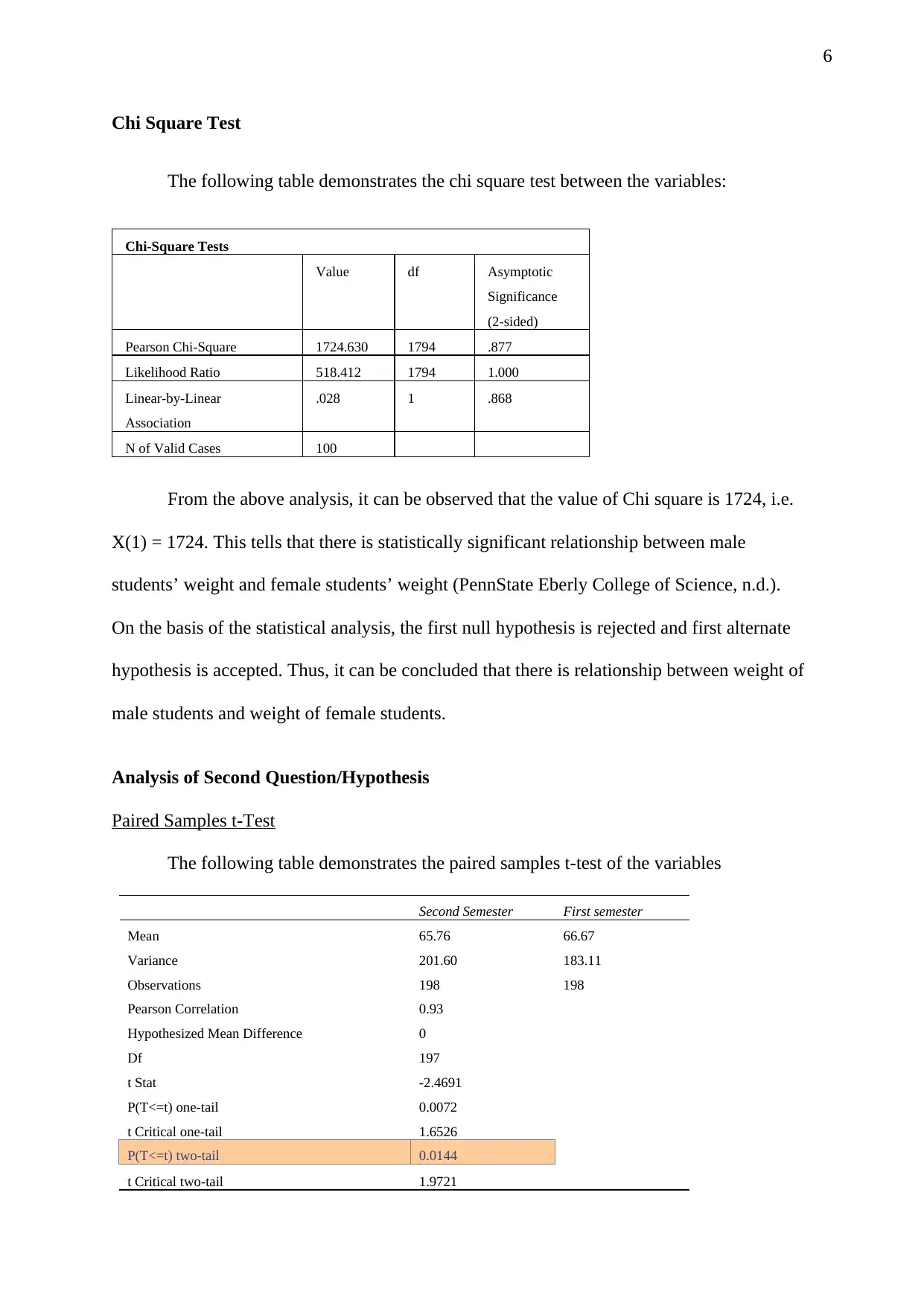
6
Chi Square Test
The following table demonstrates the chi square test between the variables:
Chi-Square Tests
Value df Asymptotic
Significance
(2-sided)
Pearson Chi-Square 1724.630 1794 .877
Likelihood Ratio 518.412 1794 1.000
Linear-by-Linear
Association
.028 1 .868
N of Valid Cases 100
From the above analysis, it can be observed that the value of Chi square is 1724, i.e.
X(1) = 1724. This tells that there is statistically significant relationship between male
students’ weight and female students’ weight (PennState Eberly College of Science, n.d.).
On the basis of the statistical analysis, the first null hypothesis is rejected and first alternate
hypothesis is accepted. Thus, it can be concluded that there is relationship between weight of
male students and weight of female students.
Analysis of Second Question/Hypothesis
Paired Samples t-Test
The following table demonstrates the paired samples t-test of the variables
Second Semester First semester
Mean 65.76 66.67
Variance 201.60 183.11
Observations 198 198
Pearson Correlation 0.93
Hypothesized Mean Difference 0
Df 197
t Stat -2.4691
P(T<=t) one-tail 0.0072
t Critical one-tail 1.6526
P(T<=t) two-tail 0.0144
t Critical two-tail 1.9721

7
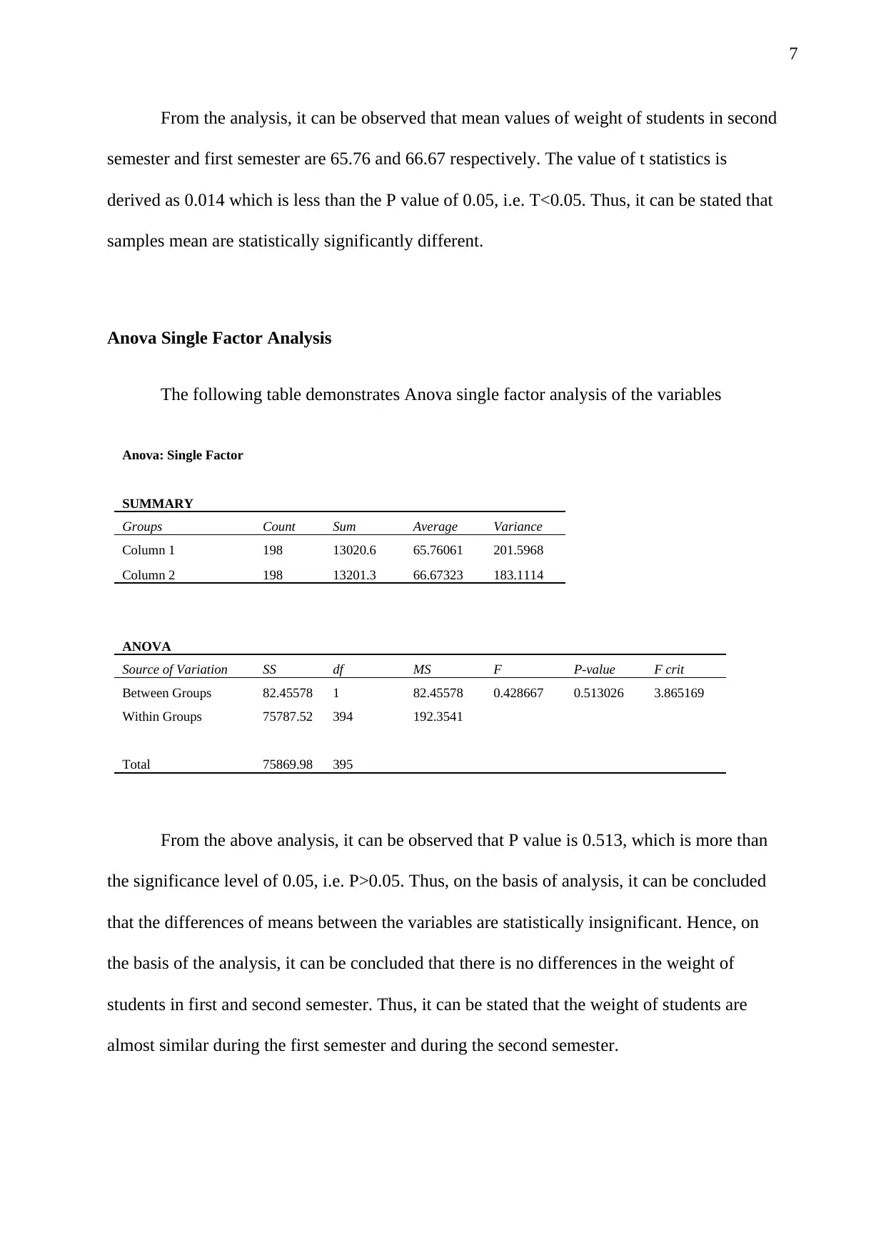
From the analysis, it can be observed that mean values of weight of students in second
semester and first semester are 65.76 and 66.67 respectively. The value of t statistics is
derived as 0.014 which is less than the P value of 0.05, i.e. T<0.05. Thus, it can be stated that
samples mean are statistically significantly different.
Anova Single Factor Analysis
The following table demonstrates Anova single factor analysis of the variables
Anova: Single Factor
SUMMARY
Groups Count Sum Average Variance
Column 1 198 13020.6 65.76061 201.5968
Column 2 198 13201.3 66.67323 183.1114
ANOVA
Source of Variation SS df MS F P-value F crit
Between Groups 82.45578 1 82.45578 0.428667 0.513026 3.865169
Within Groups 75787.52 394 192.3541
Total 75869.98 395
From the above analysis, it can be observed that P value is 0.513, which is more than
the significance level of 0.05, i.e. P>0.05. Thus, on the basis of analysis, it can be concluded
that the differences of means between the variables are statistically insignificant. Hence, on
the basis of the analysis, it can be concluded that there is no differences in the weight of
students in first and second semester. Thus, it can be stated that the weight of students are
almost similar during the first semester and during the second semester.

8
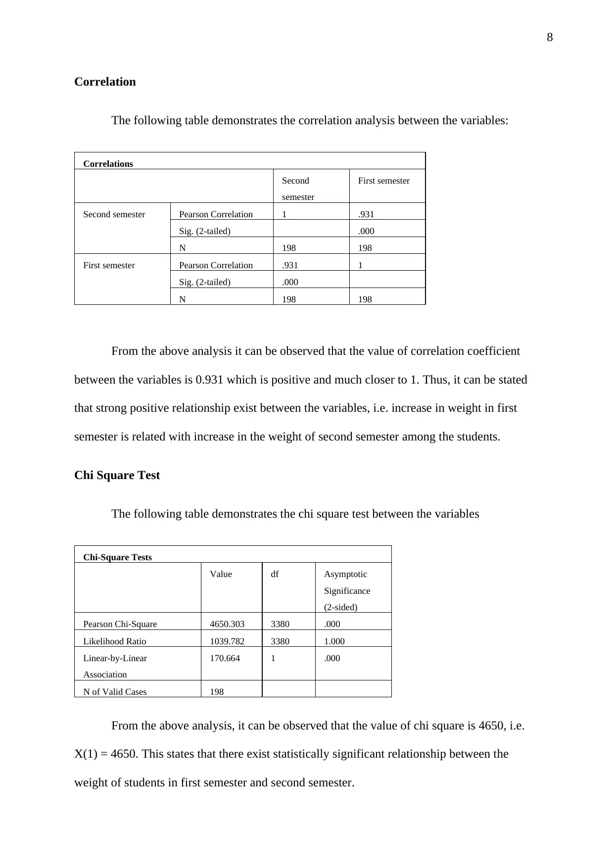
Correlation
The following table demonstrates the correlation analysis between the variables:
Correlations
Second
semester
First semester
Second semester Pearson Correlation 1 .931
Sig. (2-tailed) .000
N 198 198
First semester Pearson Correlation .931 1
Sig. (2-tailed) .000
N 198 198
From the above analysis it can be observed that the value of correlation coefficient
between the variables is 0.931 which is positive and much closer to 1. Thus, it can be stated
that strong positive relationship exist between the variables, i.e. increase in weight in first
semester is related with increase in the weight of second semester among the students.
Chi Square Test
The following table demonstrates the chi square test between the variables
Chi-Square Tests
Value df Asymptotic
Significance
(2-sided)
Pearson Chi-Square 4650.303 3380 .000
Likelihood Ratio 1039.782 3380 1.000
Linear-by-Linear
Association
170.664 1 .000
N of Valid Cases 198
From the above analysis, it can be observed that the value of chi square is 4650, i.e.
X(1) = 4650. This states that there exist statistically significant relationship between the
weight of students in first semester and second semester.

9
Thus, on the basis of the analysis, the second null hypothesis is rejected and alternate
hypothesis is accepted. Hence, it can be stated that there is relationship between the weight of
students in first semester and second semester.
Conclusion and Recommendation
The key findings obtained from the research are that the average weight of male
students is higher than average weight of female students. Furthermore, there exist certain
relationship between male students’ weight and female students’ weight. On the other hand, it
has also been found that weight of students is quite similar between first and second semester.
Besides, certain positive relationship has also been found between the weights of students in
both semesters. This research calls for better analysis and quality of reporting with respect to
weight gain. Reported information should be presented with standard deviation for properly
interpreting the findings. Moreover, beyond the overall weight changes, the proportion of
students gaining weight require to be reported for better evaluation.

10
References
Halls. (2017). What is BMI? Retrieved from http://halls.md/bmi-difference-men-women/
Heiman, G. (2010). Basic Statistics for the Behavioral Sciences. Cengage Learning.
Peck, R. (2015). Introduction to Statistics and Data Analysis. Cengage Learning.
PennState Eberly College of Science. (n.d.). 4.0 - Chi-Square Tests. Retrieved from
https://onlinecourses.science.psu.edu/statprogram/node/158
Sharma, J. K. (2007). Business Statistics. Pearson Education India.
Sreejesh, S. (2013). Business Research Methods: An Applied Orientation. Springer Science &
Business Media.
Vadeboncoeur, C. (2015). A meta-analysis of weight gain in first year university students: is
freshman 15 a myth? BMC Obesity, 2(22), 1-9.